Error Spending in Sequential Testing Explained

Sequential analysis of experimental data from A/B tests has been quite prominent in recent years due to the myriad of Bayesian solutions offered by big industry players. However, this type of sequential analysis is not sequential testing proper as these solutions have generally abandoned the idea of testing and therefore error control, substituting it for what seems like an ersatz decision-making machine (see Bayesian vs Frequentist Inference for more on this).

Frequentist sequential testing on the other hand is becoming more popular by the day with the reasons being twofold. On the one hand CRO experts, product managers, growth experts, and analysts are becoming more aware of the adverse impact of the misuse of significance tests and confidence intervals that we call peeking. In short, peeking with intent to stop breaks the validity of both risk estimates and effect size estimates and largely defeats the very purpose of A/B testing.

On the other hand, being able to analyze test data as it gathers and to act on it swiftly has many benefits as long as one can maintain the desired error control throughout the process. See the sequential testing entry of our glossary and the articles linked there for more details on both the benefits and the drawbacks to sequential hypothesis testing.

Sequential testing is based on a concept called error spending which is what allows us to make statistical evaluations of the data continuously or at certain intervals (predefined or not) while retaining the error guarantees you would expect from a frequentist method. In this article I will try to explain error spending in an accessible manner and without going into the mathematical details. These are covered to a greater extent in chapter 10 of my 2019 book “Statistical Methods in Online A/B Testing” and the cited literature.

Why do we need error spending?

To answer this and other questions I will make ample use of simulations and visual aids. Axis ranges are deliberately kept the same across comparable graphs to aid in direct visual comparisons (exception: right y-axis of graph #2 is very slightly off in order to keep the left y-axis the same).

Let us say we plan to run a test and evaluate its data at 12 monitoring points equally spaced in time. You can think of it as a test running for 12 weeks, for example. We have chosen a 0.05 p-value threshold.

Furthermore, we will use a simple rule to decide when to stop (stopping rule): if at a given monitoring stage the p-value for the difference between B (treatment) and A (control) is lower than the chosen significance threshold, we stop the test and declare the variant a winner. This rule is equivalent to stopping the experiment when a one-sided 95% confidence interval for difference in proportions excludes zero.

Using the above rule is equivalent to unaccounted peeking with intent to stop. Plotted on a graph this stopping rule looks like so:

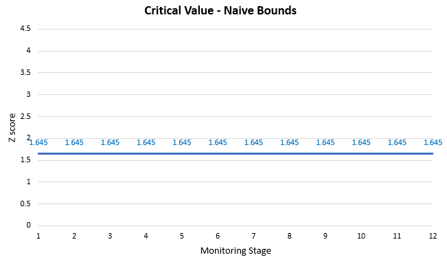
A Z score of 1.6448 corresponds to our chosen 0.05 one-sided significance level and we compare the observed p-value with the same 1.6448 value at each monitoring stage. Nominally the test has a 0.05 error rate (5% type I error rate). But what is the actual error rate?

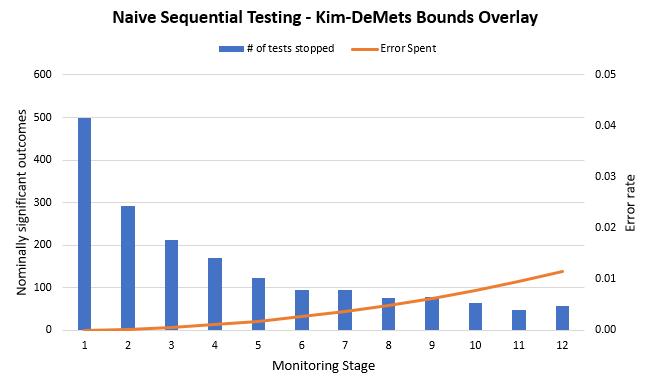
On the graph below you see the results from 10,000 simulation runs in which A/A test data was evaluated at 12 equally-spaced points in time. A/A means there was zero actual difference between the treatment and control groups so all observed discrepancies are due to what we model as random noise. Due to the random error we get 10,000 sample paths, some of which lead to large observed differences at different points in time.

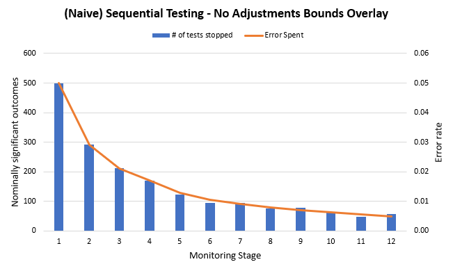
The graph shows the number of tests declaring a winner at each stage (columns) as well as the error probability spent on each stage (line). There are 498 winners in the very first stage, which is what one would expect from a procedure with up to 5% error probability (498/10000 = 4.98%). However, this is just one possible outcome! If the error rate is to be maintained across the whole set of possible outcomes from the test (all outcomes on all possible exit stages), we would have to see zero tests declare a winner for stages two through to and including twelve.

But that is not the case. There is a declining number of positive outcomes. The reason the number is not steady is that tests reaching later stages partially depend on outcomes of tests on previous stages. The ones showing the greatest discrepancies gradually end as the test reaches later stages which has a double effect of reducing the total number of tests reaching each subsequent stage and also making it less and less probable that these tests would show large enough differences to reach the critical value we have set. That is why despite the critical value being flat it results in a convex error spending line.

If we sum up all tests in which a nominally significant result was observed at any stage, we get 1804 false positives out of 10,000 tests or a rate of 0.1804 (18.04%). That is roughly 3.6 times larger than the target rate of 0.05 (5%).

Note that the same result can be achieved if we sum up the probabilities expressed by the error spent line. In effect, by using this naive rule we actually applied a spending function of the shape shown on the graph.

The issue is – this spending function is no good as it doesn’t preserve the error guarantees we want. Whether we use this error spending function to control type I error (alpha spending) or type II errors (beta spending), the actual error rates it will produce will be far away from the target ones. Simply put, we will be greatly mislead as to the uncertainty of any estimate.

What would a proper error spending function look like?

Understanding the problem, now let us try to imagine what a good error spending function would have to do to the above outcomes in order to preserve error control.

First, it would need to reduce the number of type I errors observed on the first stage so that there is some potential for errors left for the later stages. If it doesn’t do that, then it is equivalent to a classic fixed sample design with a single evaluation point.

Second, it should smear the remaining error probability across stages 2 to 12 in such a manner, that when you sum up the error probabilities across all stages they add up to the nominal rate. In this case that’s 0.05, but it can be any other number.

Visually, it should cut short some or all of the columns on the graph above and redistribute parts of them to other stages.

As a metaphor, think about making a plastic bow using a press mold. You can think of the false positives as plastic material which is several times in excess of what’s required. Not only that, but it is also spread very unevenly. The spending function is the press mold which should shape a bow from that initial condition. When you press on the plastic, the excess is squeezed out and the remaining ones are ordered in the shape of the mold. When you apply a spending function it removes excess type I errors and reorders the rest across the monitoring stages.

A simple error spending function (Pocock bounds)

Knowing the above, what would be the simplest way to press on the graph so as to reduce and smear the errors across the stages? Surely, if we just lower the significance threshold (raise the confidence level) enough evenly across all stages that will produce an error spending which controls the error rate at the desirable level. We’ve just reinvented the Pocock spending function, originally the Pocock multiple testing bounds named after their inventor Stuart Pocock ^[1].

A plot of the critical values produced by that spending function is shown below:

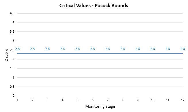
Pocock’s approach is to simply raise the critical value from 1.6448 to 2.3 at all evaluation stages of the A/B test. Using a Z-score to p-value calculator can tell us that is equivalent to a significance threshold of 0.0107 (98.93% confidence level) on each stage. Visually that would look like so (blue bars are from the initial simulation still):

The function would achieve what was described as desirable properties in the previous section. First, it would vastly reduce the number of false positives on all stages. Second, it will spread the remaining error probabilities more evenly across stages, though a slightly larger number of them would still be concentrated in the early stages.

The simplicity of Pocock’s approach has its drawbacks as well. Most notably, due to concerns for the external validity of the A/B test outcomes it is usually not desirable to stop tests so early on even if the results are statistically valid. This is the reason several other types of multiple testing procedures were proposed in a span of several years to several decades following his work, a prominent example being the work of O’Brien and Fleming just two years later ^[2] and others as discussed in chapter 10 of “Statistical Methods in Online A/B Testing”.

Advanced spending functions (Kim & DeMets)

Without getting into why and how statistical methods evolved from bounds calculated at exact moments in a test to spending functions, I’d like to introduce the alpha spending function used in the AGILE A/B testing method put together and popularized by myself in recent years ^[3]. This function is also used in our sequential A/B testing calculator. It is but a particular instance of the alpha spending functions introduced by Kim & DeMets ^[4] , also known as Kim-DeMets power functions.

With a power of 3 the function results in a downward sloping set of Z score boundary values:

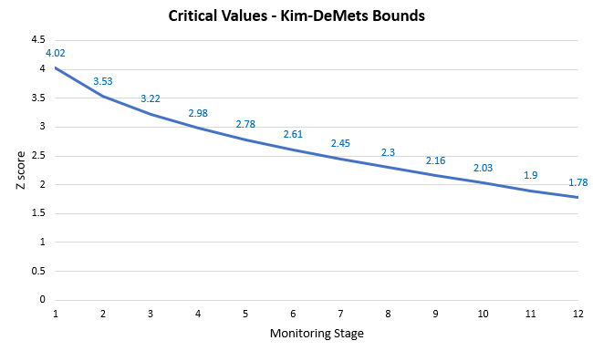
You can get an idea of how it cuts and presses on or smears the outcomes of peeking by examining the graph below (blue bars are from the initial simulation run):

As you can imagine, applying such a ‘press mold’ would result in a set of outcomes quite different from both the naive peeking as well as the Pocock function.

Rerunning the simulation using this new stopping rule instead of the peeking that we did initially, one can see how different the distribution of the outcomes is:

As you can see, using the ‘press mold’ shaped by the Kim-DeMets spending function resulted in squeezing out the majority of the false positives. This reduces the overall number of type I errors so the test ends up controlling the error rate at the target 0.05 level. The function smeared the rest of the error probability in a way which allocated near-zero error probability in the early stages of a test. It becomes move permissive at later stages.

The conservative nature of this error spending function in the early stages is in alignment with the goal of achieving not only internal validity (statistical validity), but also good external validity (generalizability) of the outcomes of an A/B test.

See this in action

Try itA/B Testing Hub
The all-in-one A/B testing statistics solution

Summary and endnotes

This article introduced the need for error-spending functions and briefly explained how an error spending function works and why it is the right way to ‘peek’ at data in an efficient yet statistically rigorous way. It is deliberately light on mathematics so I hope it achieved the goal of introducing the concept in a way somewhat more accessible to non-statisticians.

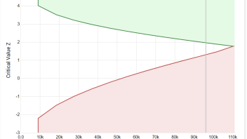
The concept of error spending functions was examined by focusing particularly on examples of alpha spending ones. However, the same logic can and has been extended to beta spending for type II error control. In fact the use of futility bounds is one of the main selling points of the AGILE test design. Shown below is one such design with the green line being the boundary constructed by alpha spending and the red line the boundary constructed by beta spending:

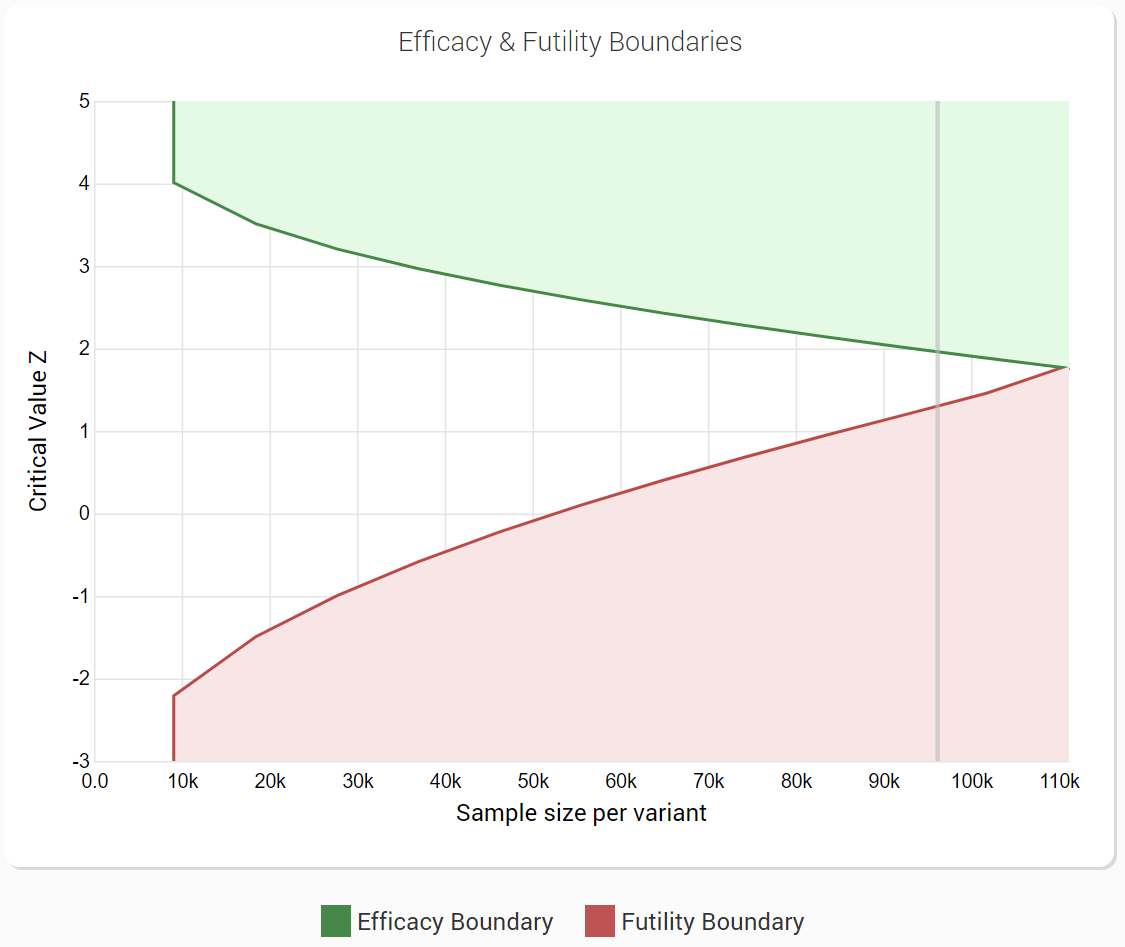
While the particular efficiency gains achieved by using sequential testing instead of fixed sample size tests are not the topic of this article, they are very significant especially when both efficacy and futility stopping boundaries are used. Edit: As of 2024 this topic is explored in a meta-analysis of 1001 A/B tests (see the section on “Efficiency of Sequential Testing”). The efficiency of alpha and beta spending in relationship to other popular sequential tests is explored in “Comparison of the statistical power of sequential tests: SPRT, AGILE, and Always Valid Inference”.

For more details on sequential testing see my white paper, the many blog posts as well as my aforementioned book.

References

1 Pocock, S.J. 1977. “Group sequential methods in the design and analysis of clinical trials.” Biometrika 64: 191–199. doi:10.2307/2335684.
2 O’Brien, P.C., and T.R. Fleming. 1979. “A Multiple Testing Procedure for Clinical Trials.” Biometrics 35: 549–556. doi:10.2307/2530245.
3 Georgiev, G.Z. 2017. “Efficient A/B Testing in Conversion Rate Optimization: The AGILE Statistical Method.” www.analytics-toolkit.com. May 22. Accessed May 15, 2020. https://www.analytics-toolkit.com/pdf/Efficient_AB_Testing_in_Conversion_Rate_Optimization_-The_AGILE_StatisticalMethod_2017.pdf.
4 Lan, K.K.G., and D.L. DeMets. 1983. “Discrete Sequential Boundaries for
Clinical Trials.” Biometrika 70: 659-663. doi:10.2307/2336502.

About the author