This article will examine the effects of using the HyperLogLog++ (HLL++) cardinality estimation algorithm in applications where its output serves as input for statistical calculations. A prominent example of such a scenario can be found in online controlled experiments (online A/B tests) where key performance measures are often based on the number of unique users, browsers, or devices. In A/B testing, one performs statistical hypothesis testing and estimation in order to inform business decisions. The accuracy of these statistical estimates is crucial for making correct informed choices. The article examines in detail the perils of relying on HyperLogLog++ cardinality estimates in A/B tests. The conclusions should generalize well to other algorithms with similar performance and to more complex statistical assessments, as well as to other types of statistical analyses such as regressions.
The article is structured as follows: First, I present a brief overview of what cardinality estimates are, why they may be needed and useful, and give a surface-level description of the HyperLogLog (HLL) algorithm and its accuracy. Second, I present simulation results showing the effect of using HyperLogLog++ estimates instead of exact counts in a straightforward A/B testing scenario. Finally, I offer an explanation of the results and a brief discussion.
What are cardinality estimates?
The increasing availability of big data in the past several decades gave rise to the need for fast computation of the cardinality of various data sets. For example, such computations are required when one needs to know the number of unique users visiting a website over a particular time frame, the number of unique mobile devices to which an ad was shown during an advertising campaign, the number of unique IP addresses which accessed a given network resource, etc.
A combination of hardware limitations (available storage) and performance requirements mean that exact count approaches become unfeasible in certain situations and so various probabilistic approaches were developed to offer fast and fairly accurate estimates with minimum resource utilization.
It should be noted that cardinality here is used not in the strict mathematical meaning synonymous to “number of elements in a set”, but in the SQL-related meaning where cardinality refers to the uniqueness of the values contained within a given database column. In particular, it will be used synonymously with “number of unique elements in a set”.
For example, if a database contains 1,000 rows each of which has a column named “User ID” which contains unique user identifiers, the “User ID” column has a cardinality of 1,000. If another database contains 10,000 rows representing one session each, its “User ID” column would contain repeated values and will have a cardinality of less than 10,000 if at least one user has had more than one session.
Why is it difficult to estimate the cardinality of a data set?
The main difficulty in counting the unique (distinct) values in a set comes from the need to store a table of all unique values. If such a table is not stored, then recalculating the cardinality when new rows are added to the data set would require revisiting each and every row of the source data in order to calculate it on the fly, which in most cases is too expensive for big, continuously updated datasets.
When the data set is expected to be fairly small, getting an exact count of the number of unique values in a given column is easy and done through hash maps or zero-collision bit maps. The latter are much more compact than the former, but still require substantial storage and a good guess about the cardinality of the data which makes them impractical in many cases.
When the above options become unsuitable, one approach is to sample some of the data in order to try and estimate its cardinality. The issue with that is that the sampling error is unbounded and can vary greatly depending on the ratio of the sample size to the total size of the data set, as well as when the values exhibit clustering. Sampling approaches are therefore not very practical.
Sketch-based algorithms and HyperLogLog
The last family of estimates is the one to which the HyperLogLog algorithm belongs. Some of the earliest examples of such approaches were described in 1985 [3], but currently the most prominent algorithm is HyperLogLog which was designed by Flajolet et.al. in 2007 [1], and later improved upon by Google’s Huele et.al. in 2007 [2] (dubbed HyperLogLog++) and further by Ertl in 2017 [4]. The general approach is to make observations on the hashed values of the input multiset elements in order to reduce the size of synopses (sketch). The usual choice is a prefix in the binary representation of the hashed values of a particular length. In HyperLogLog this is done by first storing the logarithmic hash values in prefix-based buckets (called registers) and finally by computing the harmonic mean of the maximum count of leading zeroes across all such buckets.
These observations are independent of both replication and order of the items in the dataset which results in an unbiased estimate with a fairly constant size of the relative error across a wide range of cardinalities (especially true for [3] and [4]).
Another key advantage is that the size of the sketch is extremely small relative to the number of unique values for which the estimate is made e.g. a few Kilobytes for one billion unique values. HyperLogLog and its improvements are also faster in indexing the data than all alternatives [3]. Merge operations and hence updating the estimate are also quite efficient.
If you are interested in the finer details of how the estimation algorithm works, I invite you to go through the references below as well as to check out a publicly shared presentation by Andrew Sy titled “HyperLogLog – A Layman’s Overview”.
How accurate is HyperLogLog++?
The original HyperLogLog algorithm offers a fairly constant relative standard error across a range of cardinalities with a standard deviation (σ) equal to:
σ = 1.04 · √m
where m is the number of registers (e.g. 1, 2, 4, … 1024, 4096, 16384, 65536). For example, with 12-bit registers m = 212 = 4096 and the relative error is 1.625% while with 16-bit registers m = 65536 and the error is 0.40625%. This means that the estimated value of 68% of cardinality estimates would be within ±0.40625% of the true cardinality.
The original HyperLogLog suffers from increased inaccuracy for cardinalities between approximately 30,000 and 60,000 which is addressed in HyperLogLog++ [2]. The same work also introduces sparse representation which results in the error being multiple times smaller for true cardinalities below 12,000.
While Ertl 2017 [4] and several others claim improvements over both HLL and HLL++, it is the latter which has seen adoption in major database applications (e.g. Redis, Spark, Presto, Riak) and in analytics products by major corporations (e.g. Google Analytics, Google BigQuery, Adobe Analytics, and others). This plus the availability of error distribution data is why HyperLogLog++ will be the focus of the next parts of the article.
Figure 8 in Heule et.al. (2013) [2] shows that the median relative error in absolute terms is approximately 0.005 (0.5%) with a 95% quantile close to 0.015 (1.5%) and the 5% quantile around 0.0005 (0.05%) for true cardinalities in the range 60,000+. The large exception is for values under 12,000 for which the median error is 0.001 (0.1%), but these would not be of interest in this article. Similar results are obtained by Harmouch et.al. (2017) [3].
This accuracy might seem excellent at a first glance. It is, indeed, completely adequate for many applications. However, as shall be demonstrated in the next part, such an inaccuracy can have dire consequences when introduced into statistical analyses such as those performed in A/B tests.
Simulated Statistical Analyses Based on HyperLogLog++ Estimates
The simulation is based on a scenario of conducting A/A tests with a user-based proportion measure for which the number of users is a HyperLogLog++ estimate. The measure can be any kind of user-based conversion rate, e.g. Average Transactions/Purchases Per User (assuming one transaction/purchase maximum).
It is further assumed that the number of events (transactions, purchases, etc.) is extracted as an exact count. The above is realistic since such events are usually much smaller than the number of users, and furthermore have a unique ID so an exact count is usually easy to obtain.
The whole simulation mimics the experience of a marketer or user experience specialist using Google Analytics data in online experiments.
Approximating the HLL++ error distribution
Since my goal here is to be able to quickly run many simulations with different cardinalities and not to make a super exact assessment of HLL++, I’ve decided to use an approximation of the error distribution. The Beta distribution with parameters α = 1.5 and β = 260 seems to offer a reasonably close approximation. It has a median of approximately 0.4476%, 95% quantile of 1.502%, a 99% quantile of 2.1756%, and a 5% quantile of 0.0685%.
set.seed(100)
nums = rbeta(10000, 1.5, 260); hist(nums, xlim = c(0,0.02), breaks = seq(0.0,1,by=0.001), freq=FALSE);
quantile(nums, c(0.05, 0.5, 0.95, 0.99))
Here is a histogram of that distribution (click for full size):
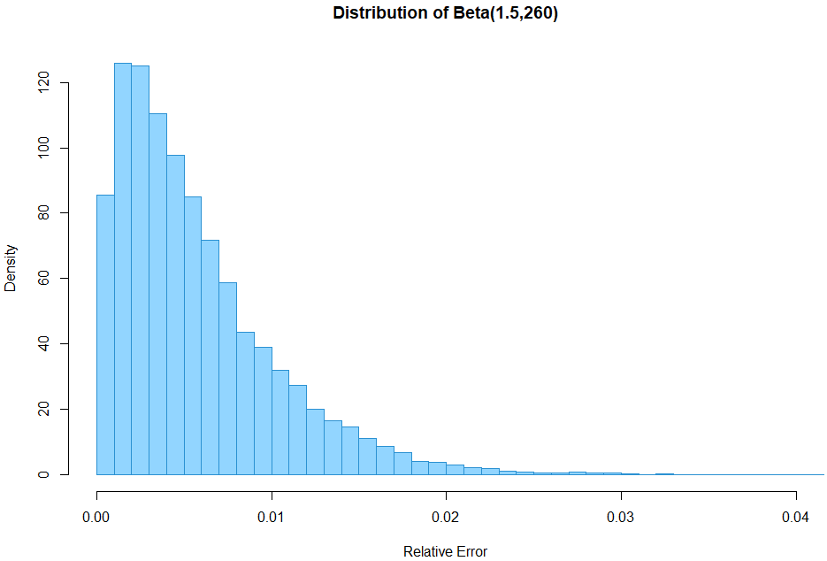
It may actually be conservative when compared to the Huele et.al. quantiles above due to the 10% smaller median error so it should be a fair enough representation of the actual HLL++ error rate.
HyperLogLog++ A/A Test Simulation Results
Running the code from Appendix 1 with six different cardinalities: 20,000, 50,000, 100,000, 200,000, 500,000, and 1,000,000, resulted in the following p-value distributions (click for full size):
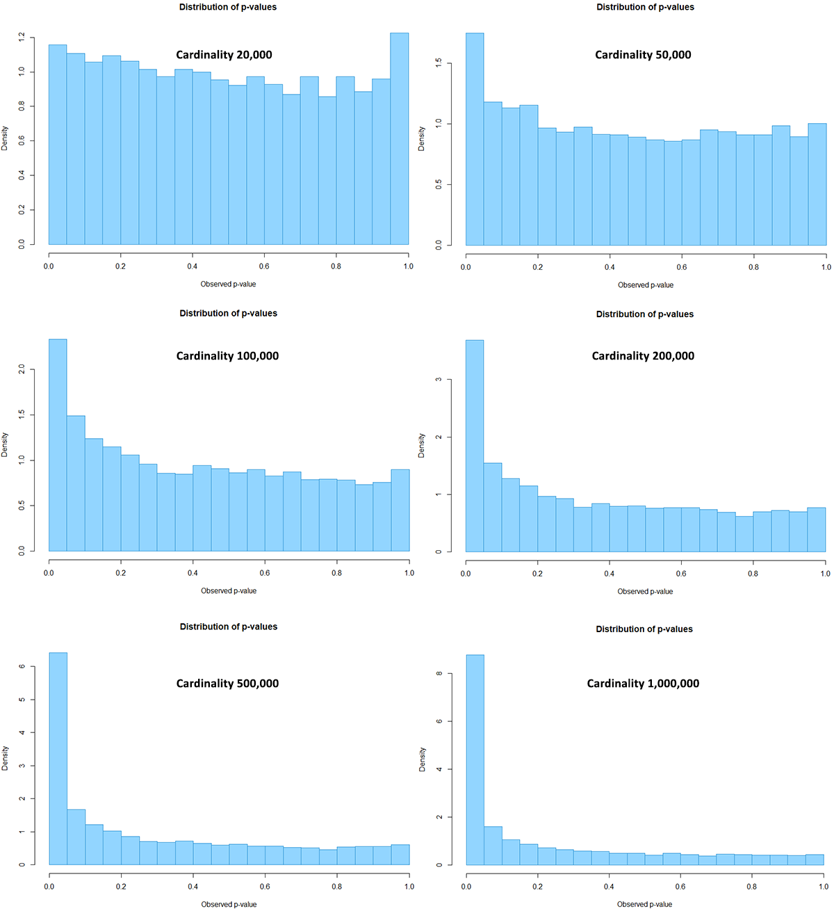
Visible, but small discrepancies from the expected uniform distribution are present even with actual cardinality of 20,000. Larger departures from the expectation become apparent with 50,000 users. The distribution becomes enormously skewed when the cardinality reaches 1,000,000.
Below is a table with expected versus observed proportions of p-values falling below several key thresholds at different true cardinalities:
| Cardinality | P-values below 0.05 | α inflation | P-values below 0.01 | α inflation | P-values below 0.001 | α inflation |
| 20,000 | 5.79% | 16% | 1.50% | 50% | 0.17% | 70% |
| 50,000 | 8.75% | 75% | 2.57% | 157% | 0.45% | 350% |
| 100,000 | 11.67% | 133% | 4.39% | 339% | 1.00% | 900% |
| 200,000 | 18.43% | 269% | 8.41% | 741% | 2.76% | 2660% |
| 500,000 | 32.11% | 542% | 19.29% | 1829% | 9.85% | 9750% |
| 1,000,000 | 43.86% | 777% | 31.97% | 3097% | 20.67% | 20570% |
| 5,000,000 | 71.04% | 1320% | 62.49% | 6149% | 53.07% | 52970% |
The proportion of p-values below any given alpha (α) threshold increases with an increase in cardinality and so does the inflation of the actual versus the nominal type I error rate. A visual presentation of the relationship between actual sample size and alpha inflation is shown on the chart below (click for full size).
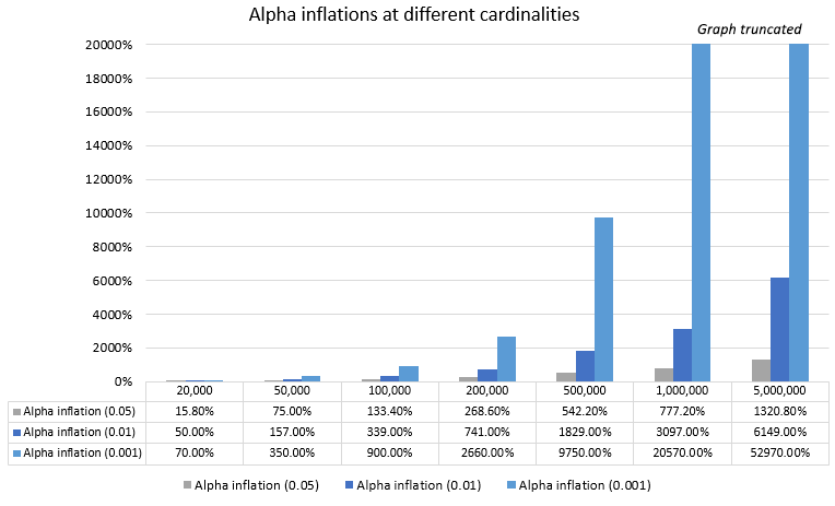
Arguably, such extreme discrepancies (starting from 0.16x for α = 0.05 with 20,000 users and reaching 13x for α = 0.05 with 5 million users) between actual and nominal statistical estimates are unacceptable in any scenario. If one prefers a more strict evidential threshold like α = 0.01 then it will be relatively severely compromised even at the smallest cardinality value (20,000 users) with a 50% increase in actual vs. nominal type I error rate. It only gets worse with decreasing the threshold and increasing the cardinality.
Sample Ratio Mismatch (Goodness-of-Fit) Results
Sample ratio mismatch (SRM) is a common indicator for issues with the setup of an online experimentation platform. Issues caused by a variety of reasons can be detected by means of a Chi-Square goodness-of-fit test for the observed versus the expected ratio between the test groups’ sample sizes.
The SRM tests from the simulated HLL++ data resulted in the following p-value distributions (click for full size):
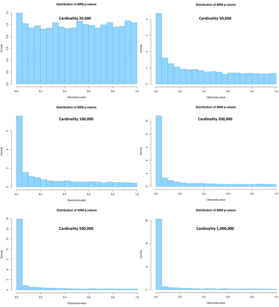
At the lowest cardinality there is a small departure from the uniform distribution. With a sufficiently high p-value one would discard tests invalidated by the inaccuracy introduced by HLL, but such high p-values are rarely used in practice since this would entail significant undesirable overhead on the testing program.
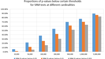
Below is a table with the proportion of tests with p-values below several key thresholds:
| Cardinality | SRM P-values below 0.05 | SRM P-values below 0.01 | SRM P-values below 0.001 |
| 20,000 | 6.00% | 1.78% | 0.39% |
| 50,000 | 21.79% | 11.63% | 5.19% |
| 100,000 | 37.93% | 25.30% | 15.49% |
| 200,000 | 54.05% | 42.04% | 30.49% |
| 500,000 | 69.95% | 61.52% | 51.81% |
| 1,000,000 | 77.03% | 70.21% | 63.18% |
| 5,000,000 | 89.42% | 86.35% | 82.73% |
It is apparent that as the cardinality increases the probability of discarding a test even at stringent p-value thresholds such as 0.001 becomes quite high. This is due to the higher power of the Chi-Square test with increases in sample size.
Here is a visual representation of the same set of mis-specification tests:
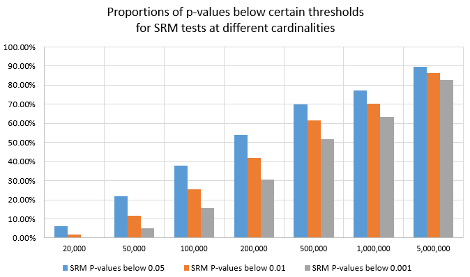
for SRM tests at different cardinalities
This is a confirmation that the sample ratio mismatch test is a powerful tool for detecting issues with the testing setup, even when these are as subtle as the use of cardinality estimates in place of exact counts of unique users, browsers, devices, IPs, etc.
Discussion: Is HyperLogLog Data Admissible for Statistical Analyses?
As a solution for obtaining unique counts of high cardinality data sets, HyperLogLog++, arguably, is supposed to be most useful when the number of unique set elements is the highest. Yet it is there where it fails the most in serving data of sufficient accuracy for statistical applications.
This behavior is due to the constant relative error characteristic of the algorithm. The statistical estimate expects higher and higher precision with increasing numbers, but instead the HLL++ algorithm results in larger and larger absolute errors. With increasing numbers of data points the accuracy of the data set is in fact decreasing or remains constant which means it offers a poorer basis for statistical analysis. This leads to statistical estimates which have worse and worse actual accuracy the more data there is – a paradoxical situation.
Note that in this simulation the error distribution is fixed across all cardinalities whereas in reality it increases slightly between 0 and ~100,000.
It is obvious that gathering more HLL++ data in the above scenario does not lead to the normally expected decrease in the uncertainty of the statistical estimates. For this reason I think HyperLogLog data with precision typical of current default implementations is unsuitable for use in A/B testing and similar scenarios where an estimator is supposed to converge to the true value in the asymptotic case. Adjusting the statistical estimates so that they account for the inaccuracy introduced by HLL++ would simply make them incredibly inefficient, therefore thwarting the very purpose of statistics which is the efficient use of data. It is also possible that such attempts may lead to a situation in which even infinite data is not enough to reach key thresholds.
I believe users of databases and analytics solutions that rely on or offer support for HyperLogLog++ and similar cardinality estimates should be aware of the above before they turn to using them for statistical analyses. The mileage of different users will vary depending on the particular implementation of HyperLogLog. For example, Google Analytics users enjoy an inaccuracy of up to 2% for 99% of estimates which should match closely with the simulation results presented above whereas Adobe Analytics users suffer from a much greater inaccuracy of up to 5% for 95% of estimates (as stated in Analytics Components Guide > Reference: advanced functions > Approximate Count Distinct (dimension) as of Oct 2020). See The Perils of Using Google Analytics User Counts in A/B Testing for a more in-depth look into the issue as it plays out in Google Analytics in particular.
One possible way out of this while still using HyperLogLog is to do so with significantly greater precision. If the registers use prefixes with significantly greater number of bits, then the accuracy of the estimates can be improved to a point where it no longer has a negative impact on A/B test outcomes even for larger cardinalities. That obviously comes with the drawback of much larger sketch sizes. How much precision is required for each scenario needs to be estimated on a case-by-case basis.
References:
1 Flajolet P., Fusy É., Gandouet O., Meunier F. 2007. “Hyperloglog: The analysis of a near-optimal cardinality estimation algorithm.” Analysis of Algorithms : 127–146.
2 Heule S., Nunkesser M., Hall A. 2013. “HyperLogLog in practice: algorithmic engineering of a state of the art cardinality estimation algorithm.” Proceedings of the International Conference on Extending Database Technology : 683-692. DOI: 10.1145/2452376.2452456
3 Harmouch H., Naumann F. 2017. “Cardinality estimation: an Experimental survey.” Proceedings of the VLDB Endowment 11(4): 499–512. DOI: 10.1145/3186728.3164145
4 Ertl, O. 2017. “New cardinality estimation algorithms for HyperLogLog sketches.” ArXiv, abs/1702.01284.
Appendix 1: R Simulation Code
sizes = c(20000,50000,100000,200000,500000,1000000,5000000);	# add/remove values to explore different sample sizes per test arm
set.seed(100);
sims = 10000										 	# change to alter the number of simulation runs
n = sizes[1];											# change the index to choose how many samples to simulate per test arm
p = numeric(sims)
srmp = numeric(sims)
for(i in 1:sims)
{
	sign1 = floor(runif(1,min=0,max=2))
	if (sign1 == 0) { sign1 = -1 }
	else if (sign1 == 1) { sign1 = 1 }
	sign2 = floor(runif(1,min=0,max=2))
	if (sign2 == 0) { sign2 = -1 }
	else if (sign2 == 1) { sign2 = 1 }
	x = rbinom(n = n, size = 1, prob = 0.1)
	y = rbinom(n = n, size = 1, prob = 0.1)
	evx = sum(x == 1)
	evy = sum(y == 1)
	ssx = n * (1 + sign1 * rbeta(1, 1.5, 260))
	ssy = n * (1 + sign2 * rbeta(1, 1.5, 260))
	z = prop.test(c(evx,evy),c(ssx,ssy),alternative="two.sided")
	p[i] = z$p.value
	srm = chisq.test(c(ssx,ssy), p = c(1/2, 1/2))
	srmp[i] = srm$p.value
}
#prints the percentage of sim runs falling below a given p-value threshold
thresholds = c(0.05, 0.01, 0.001, 0.0001)
for (i in thresholds)
{
	print(paste('Below', i, ':', sum(p < i) / sims * 100))
}
#displays histogram and quantile values
hist(p, main="Distribution of p-values", xlab=("Observed p-value"), freq=FALSE)
quantile(p, c(0.0001, 0.001, 0.01, 0.05, 0.5, 0.95, 0.99, 0.999, 0.9999))
#prints the percentage of sim runs falling below a given SRM p-value threshold
thresholds = c(0.05, 0.01, 0.001, 0.0001)
for (i in thresholds)
{
	print(paste('Below', i, ':', sum(srmp < i) / sims * 100))
}
#displays histogram and quantile values
hist(srmp, main="Distribution of SRM p-values", xlab=("Observed p-value"), freq=FALSE)
quantile(srmp, c(0.00001, 0.0001, 0.01, 0.05, 0.5, 0.95))
About the author

Managing owner of Web Focus and creator of Analytics-toolkit.com, Georgi has over twenty years of experience in online marketing, web analytics, statistics, and design of business experiments for hundreds of websites.
He is the author of the book "Statistical Methods in Online A/B Testing", of white papers on statistical analysis of A/B tests, and has been a speaker at conferences, seminars, and courses. Georgi has been distinguished as a winner in the Data & Analytics category of the 2024 Experimentation Thought Leadership Awards.

