The Bane of AB Testing: Reaching Statistical Significance

Now, this is not a new topic on this blog. I’ve discussed the issue of optional stopping based on “achieving” or “reaching” statistical significance in my Why Every Internet Marketer Should be a Statistician post more than two years ago and others have touched on it as well – both before and after me. However, the issue doesn’t seem to be going away and advice to “wait for statistical significance”, to run the test until statistical significance is “achieved” or “reached” is as prevalent as before, if not more prevalent. My observations come mainly from the advice and discussions in the conversion rate optimization industry, but I suspect the situation is not that different when it comes to A/B testing in landing page optimization, e-mail marketing, SEO and PPC.

results from tests where reaching statistical significance was the stopping rule are as real as the ship or the lighthouse above

I thought a more in-depth article was due, since as result of the continued malpractice illusory AB test results are much more common than expected and things go south for both agency/practitioner and their clients when the reported improvements (% lift) are then nowhere to be found in the business bottom-line. Frustrated, practitioners turn increasingly to “hacks” like A/A tests in an attempt to figure out what’s wrong with the results they report, but these are a waste of time and resources in the majority of cases as I argue in my Should you do A/A, A/A/B or A/A/B/B tests in CRO? post from a while ago.

In this post I’ll first describe the issue, explain some of the statistical reasoning behind and then outline a solution that goes beyond the trivial “fix your sample size in advance” advice, which is anything but trivial when attempted in practice. Instead I lay out a solution fit to the business case and applicable to all kinds of online marketing A/B and MVT tests.

Why “Reaching Statistical Significance” is Not What it Seems to Be?

or the real reason many reported A/B test results are illusory.

When initially designed, statistical tests didn’t even consider monitoring accruing data, as they were used in bio-science and agriculture where the experiments where fixed sample size worked just fine: you plant a certain number of crops with a particular genetic trait, e.g. hoping for better yield or better resistance to harmful insects and observe the result a few months or years later. Usually there is no monitoring of the results in the meantime as there were no results to monitor until the crops are harvested.

Hence the widely accepted p-value statistic, which is the basis for claiming statistical significance, is by default applicable only to cases where it is calculated after a predetermined number of observations are completed. In the case of AB testing this would be a predetermined number of users exposed to a test, whether it would be a test for a shopping cart modification, landing page variant, e-mail template or ad copy change. The statistic in its default form is nearly meaningless and has no interpretation otherwise, that is, if you peeked at the data at arbitrary or fixed times and made decisions based on the interim results.

The issue, of course, is not that you peaked, but that you made decisions to stop or continue the test before the planned stopping time based on the current results in terms of nominal p-value or statistical significance, conversion rate, CTR, etc. If you did that, then whatever statistical confidence you report can be at best worthless and at worst – misleading. This is the kind of thing that, if discovered, gets your scientific paper taken down and the results declared null and void. If you didn’t have a predetermined stopping time or sample size, then the situation is even more dire as you didn’t even had the chance to get it right.

If you did that, then whatever statistical confidence you report can be at best worthless and at worst – misleading.

If a statistician is called at this point in time he’d only be able to do a postmortem and tell you how you should do your test next time and I explain why below.

Fishing for Statistical Significance

or why the fish in your bag ain’t as representative of all the fish in the water as you think. I’ll try to explain the effect of outcome-based optional stopping on the sample space with a fishing metaphor. I find it a bit easier to grasp than coin-tosses when it comes to A/B tests, hopefully you will as well.

Let’s imagine that instead of testing conversion rate for users we’re testing bait for fish in a lake. We have two fishing rods set up, each with a different bait and we refresh the bait on each rod after we catch a fish with it. We want to see which bait results in more fish being caught per hour. Now let’s assume that there is in fact no real difference in the performance of the bait: the fish shows no preference for either. However we don’t know that, yet, so we’re fishing with both kinds of bait, hoping that one will outperform the other by some minimum margin that justifies us bothering to test, e.g. buying and handling a second kind of bait, etc.

Since fish behavior is subject to a variety of factors other than the kind of bait used, it is more or less random from the viewpoint of our test. Due to that “randomness” there is variance in how much fish we tend to catch in any given hour using each type of bait, so there will be times when one bait will outperform the other and vice versa, even though the fish has no real preference for either. The less fish we’ve caught, the more likely it is that that variance will manifest in a significant (in magnitude) difference between the observed performance of the two kinds of bait.

In an ideal world where we live forever and there are no limits to our resources we can afford to wait until we catch all the fish in the lake and then to simply count the numbers we’ve caught using the two baits and then we’d know for sure that there is no difference in their performance. In this case the observed performance will exactly equal the actual performance, so there are no uncertainties in the outcome. However we have pressures to get results now, rather than later and to get them with the least amount of effort and resources possible. That’s why we’d have to be content with a limited sample from the total behavior of the fish in the lake. This means we’d have to tolerate a certain level of uncertainty.

The level of uncertainty of our observed outcome is expressed in statistical terms as a p-value, statistical confidence, confidence interval or another statistic.*

So the smaller the p-value, the less uncertainty there is in our data. But the p-value is nothing more than a function of the observed data – how many fish we counted and how extreme the difference in effect between the two kinds of bait is (if we stick to the metaphor for just a bit more). Now, let P1 denote the probability of observing a positive difference in performance equal to or larger than some percentage δ, even if there is no positive difference, when we check our data once, after a whole day of fishing. Then let’s define P2 as denote the probability of observing a positive difference in performance equal to or larger than some percentage δ, even if there is no positive difference, at least once while we peek at the number of fish next to each rod every hour during the day (24 times).

The behavior in P1 represents a classic fixed-sample hypothesis test while the behavior in P2 corresponds to optional stopping based on observed outcomes during the test. The question is then, is P2 lower, higher or the same as P1? If it is lower or the same, then we should be able to peek with immunity. Otherwise, peeking should not even be considered an option given that some kind of error control is to be sustained.

If the fish behavior were constant, then it wouldn’t matter and P1 would be equal to P2. But if we knew the behavior is constant, we don’t really need to do any experiments, as we already know all we need to know. At worst we’d need just one observation point per fishing rod in order to determine the (constant) difference in performance.

However, as pointed out already, fish behavior is not constant – it varies, hence the more often we look the more likely we are to observe an extreme difference between the two baits at least once, even when there is no real difference. Trying and failing to observe a significant difference during multiple attempts is then, in fact, gathering evidence against the hypothesis that there are differences in the two baits. If the difference is harder to find, the chance of it existing and of being of a certain magnitude are naturally lower. Thus P2 is always higher than P1 and since P1 and P2 are in this case actually error probabilities, it turns out that our p-value should be higher if we were peeking, compared to the case were we do just one count at the end.

Since a higher p-value corresponds to a lower level of statistical significance, it means the reported nominal statistical significance or confidence levels will be garbage.

In conclusion: fishing for statistical significance results in reported error probabilities which are lower than the actual ones and thus in reported statistical confidence which is higher than the actual one. Decisions based on such statistics would not be warranted by the data with the desired level of certainty.

A more graphical illustration of the above is presented below. Imagine we are given these two graphs:

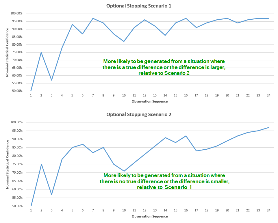
The observation sequence covers 24 observations, let’s say that’s one every hour. The blue line is the observed p-value / statistical confidence. Since the confidence is proportional to the observed difference, it is quite straightforward that the graph in Scenario 1 is more likely to have been generated from a situation where there is a higher true difference compared to the situation the graph in Scenario 2 was likely generated from.

Now, if we report only the end result and hide or disregard the valuable information that we peaked each hour and were ready to stop if significance was reached, then the two Scenarios would appear to be equally probable. However, if we take into account the fact that we were peaking, and were ready to stop if significance was reached, but we didn’t, then this information translates into much higher probability that we were in fact observing a graph like the one in Scenario 2, versus a graph like the one in Scenario 1. This is due to the simple fact that in Scenario 1 we have a much higher chance to stumble upon a moment where significance is reached, and thus never reach the 24th observation:

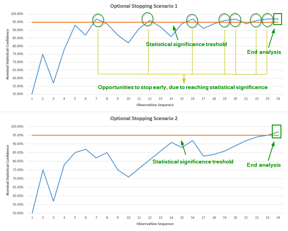
So, if we choose to ignore the information that we peaked, the two Scenarios seem equally probable. However, given we reached observation 24, Scenario 2 is in fact much more probable with peeking, as the chance we would have stopped earlier is much greater for Scenario 1. Since the graph in Scenario 2 is more likely to be generated from a situation with lower to no true difference, as compared to Scenario 1, we can deduce that performing interim analysis (peeking, fishing, waiting to achieve significance, etc.) is increasing the probability of error in our conclusion, less we adjust our statistic in order to compensate for the peeking.

Nominal vs Actual p-values and Statistical Significance

If we compare two experiments that produce exactly the same data – equal number of users and equal conversion rates, but one was stopped after “fishing for significance” and one was stopped at a predetermined number of users, they would both produce the same nominal p-value (also true for confidence intervals etc.). But we know from our fishing example above that the error probability is higher in the first case as we took more chances before making the final observation, so it was more likely that we’d see at least one significant result before reaching the number of users at which we stopped, if there was a true difference. The fact that we didn’t see one until the last observation is in fact additional data input which increases the probability that our final observation was an erroneous one, compared to the experiment with just one observation where no such data is available.

Since classical p-values are based on the assumption of just one look – at the end, failure to account for the peeking would result in one reporting the same p-values in both of the above experiments, hence we see a disconnect between the actual error probability and the reported p-value which means the reported p-value can’t be used directly to make conclusions or inferences with proper error control.

How big is this disconnect or error in reported probability? Peeking only 2 times results in more than twice the actual error vs the reported error. Peeking 5 times results in 3 times larger actual error vs the nominal one. Peeking 10 times results in 4 times larger actual error probability versus nominal error probability. The amount of disconnect is calculated by numeric integration and verified by simulations in the study by Armitage et. al.[1] which first examined the issue as far back as 1969. As you can see we are talking not in percentages, but in multiples of the nominal error probability! These are nothing to scoff at and it’s a grave issue, if left unaccounted for. This is the reason the title of the article is “The Bane of AB Testing…” and not “A Minor Issue With AB Testing…”

This is not something we can’t get around, though, as statistics has moved on since. There are methods to adjust the reported p-value so it accurately represents the error probability of our test procedure, taking into account the extra data from interim observations and analyses.

No More Illusory Results from A/B Testing

or “How to perform a statistically sound A/B test“.

There are several approaches to conducting properly designed sequential tests and for reporting accurate estimators like the observed difference, p-value or statistical significance, confidence, confidence intervals and others. I found the methods most applicable to AB testing in online marketing are the ones used in bio-statistics, medical research and trials, as well as genetics. All of them demand that the design of the test takes into account the interim observations. The methods provide rules or guidelines for stopping for efficacy at each interim analysis, while providing control of the overall level of error probability. Some methods also provide rules for stopping early for futility, or very low chance for the desired effect size.

Some of those methods provide the practitioner with significant flexibility about the time and number of interim analyses performed, mainly the ability to change the number and times of analyses as the experiments go on, depending on external factors – technical, logistical or otherwise, as well as based on observed results. E.g. you could start examining a test much more frequently than planned once you see a result which is close to being statistically significant and still maintain the desired error tolerance of the test.

See this in action

Try itA/B Testing Calculator
Advanced significance & confidence interval calculator.

There are different proposals on how to adjust estimators following a sequential test, as this is no trivial task. Fairly robust, but sometimes computationally demanding adjustment procedures are available for point estimates, confidence intervals and p-values/confidence levels.

In my brand new free white paper “Efficient A/B Testing in Conversion Rate Optimization: The AGILE Statistical Method” I go into significant detail on how one can run properly controlled tests with minimum conflict with the practical demands and pressures. We’ve also built a tool that automates the mathematical and statistical calculations and makes it easy to do analysis on the data and reach conclusions, with nice graphs for visual analysis, etc.: the A/B Testing Calculator. You’re invited to hop on the free trial we offer and try it for yourself, running new tests or testing it on data from tests already concluded.

I hope this was an interesting and light enough read into an issue that’s still plaguing the A/B testing world, partly due to lack of information, misinformation and the practices of many tool vendors to date. Unaccounted optional stopping has to end, one way or another. I’d love to hear your feedback or questions in the comment section below!

* Disambiguation for the ones interested in philosophy of science, anyone else can just skip: 

The level of certainty or uncertainty I talk about is assigned to the procedure that generated the data, the design and execution of the experiment. It would be wrong to directly infer the alternative hypothesis from a low level of uncertainty. That is, we can say that using this procedure, this method of conducting experiments or tests, we’ll only get a result as extreme or more extreme than the observed in only a given percent of possible cases, under the null hypothesis (sample space). We can’t, strictly speaking, assign a probability to a hypothesis, without making an inferential jump.

The move to inferring evidence for a hypothesis from a non-chance discrepancy requires an additional principle of evidence, which I like to express in terms of the severity principle, and I cite prof. Mayo here:

Data x₀  from a test T provide evidence for rejecting H₀ (just) to the extent that H₀ would (very probably) have survived, were it a reasonably adequate description of the process generating the data (with respect to the question).

and more generally:

Data from a test T (generally understood as a group of individual tests) provide good evidence for inferring H (just) to the extent that H passes severely with x₀, i.e., to the extent that H would (very probably) not have survived the test so well were H false.

With that in mind, I’d put forth that if we’re conducting severe tests in the above sense, then for everyday purposes and especially when communicating to non-statisticians it’s perfectly fine to frame it in probability terms as it would be understood correctly 99.9 out of 100 times regarding the inferences the combination of data & procedure warrants.

References:

1 P. Armitage, C. K. McPherson, B. C. Rowe (1969) – “Repeated Significance Tests on Accumulating Data,” Journal of the Royal Statistical Society, Series A (General), Vol. 132, No. 2, pp. 235-244a

About the author