Designing successful A/B tests in Email Marketing

The process of A/B testing (a.k.a. online controlled experiments) is well-established in conversion rate optimization for all kinds of online properties and is widely used by e-commerce websites. On this blog I have already written in depth about the statistics involved as well as the ROI calculations in terms of balancing risk and reward for optimal business results. I will link to some of these as we go along.

In this article which I’m writing in preparation for the E-commerce Email Marketing Summit I will review the basics of A/B testing in e-mail marketing covering the methods needed for conducting successful tests: both in terms of statistical design, statistical estimation, and ROI calculations. There is a large overlap with A/B tests in website CRO, with a few specifics here and there that I will point out.

KPIs in email marketing

Due to some limitations of e-mail tracking and also in the possibilities to optimize the key performance indicators (KPIs) one can use as primary or secondary outcomes in an A/B test are not as many: open rate, click rate, per recipient conversion rate, per click conversion rate, average revenue per recipient (ARPR), and average revenue per click (ARPC). Some more advanced metrics are proposed in “How to achieve higher certainty?” below.

Which KPI is relevant depends on what is being tested and the goal of the test. For example, if we are testing a subject line and we are interested in its effect on open rate, then open rate is the obvious choice. If we are interested in its effect on revenue, then average revenue per recipient (contact, subscriber) would be the correct KPI.

On the other hand, if we are testing a new newsletter, drip or promotional e-mail template and are interested in its effect on revenue, then average revenue per click would be the appropriate metric. Using average revenue per recipient will be a poor practice as it will artificially inflate the baseline by including people not actually experiencing the test.

Any experienced optimization specialist would know that a good open rate does not necessarily correlate with a good click-through rate or purchase rate. Not only that, but they can easily have a negative correlation when the expectations set in the subject line are not met in the e-mail itself or on the landing page. A blatant example would be promising a great percent off promotion and delivering only a modest one with very restricted quantity of products sold at that promotional price.

There is one other performance indicator that needs to be mentioned, which I believe will only be of interest as a secondary outcome: the unsubscribe rate of the targeted e-mail list. We would like to know if the unsubscribe rate of the tested variant(s) is worse than our control by some substantive difference. It is only a secondary outcome since we will likely not be willing to adopt a variant only on the basis of a lower unsubscribe rate, but we may be reluctant to adopt a variant which performs better in the short term but has a higher than average unsubscribe rate thus hurting our results in the long term.

The unsubscribe rate is a great example for applying non-inferiority tests and the substantive difference mentioned will be the non-inferiority margin. The non-inferiority hypothesis will be that the rate of people who do not unsubscribe is equal to or higher than the control minus the specified non-inferiority margin.

Most of the metrics discussed above are rates, so simple binomial calculations are available both when coming up with the statistical design and when analyzing the data. The only exception from this are the two revenue-based metrics for which more work is required, especially in coming up with the statistical design (see statistical significance for non-binomial metrics).

Two types of A/B testing scenarios

In e-mail marketing we can conduct two main types of tests depending on how many future e-mails are going to be informed by the test outcome. The first type is a test the outcome from which will be used only in a single email burst, for example a Black Friday email sendout. The second type is a test the outcome from which will be used for many consecutive e-mails, for example testing a new newsletter template. There is also a third scenario in which both are combined: we use the results from a series of single e-mail burst tests to make decisions for future single e-mail bursts. For example, the results from 3 Black Friday subject line tests in three consecutive years can be analyzed together to inform the length and content of next year’s e-mail.

Both types of scenarios can be analyzed using simpler, fixed-sample statistical methods as well as more advanced sequential analysis methods. The more advanced methods bring in significant improvements in the average amount of users (e-mail recipients, contacts, subscribers) you need to reach the same statistical guarantees, but they are, well, more advanced and require a bit more complex procedures and math.

Let us highlight the differences between the two types of statistical methods.

Estimating uncertainty using Fixed-Sample tests

These tests get their name from the fact that you need to fix your sample size in advance in order for the statistic to be calculated correctly. Basically, you determine the number of recipients you will send the e-mails to up front, send out the e-mails, then wait a sufficient amount of time for the action of interest to be completed: from hours to days for open rate and click rate, from several days to several months for purchases of varying sales cycle lengths.

Due to their restriction of analyzing the data just once such tests are better suited for single-burst scenarios, so let us return to our Black Friday example above and say we had a 15% click-through rate during last year’s email campaign.

This year we have 110,000 e-mails in our e-mail list and we have Black Friday next week. How do we make sure we send out an e-mail with the best click-through rate (CTR) we can achieve given we have developed two alternatives: one based on last-years e-mail and a new variant with some improvements (or so we hope)? Since we only have limited time, what we can do is sent out e-mails to two groups, each consisting of randomly selected 10,000 e-mails from our list (20,000 total, how we choose that – see below).

Note that proper randomization is key in making valid uncertainty estimates (tip: ask your A/B testing vendor, usually your ESP, about their randomization procedure). Simple methods like assigning every odd database ID to one variant and every even one to another are not random. Randomization is needed to correctly model the distribution probability of effects of unknown confounders (covariates, factors). Failing at assuring proper randomization will almost certainly introduce bias which will not be accounted for and thus render any further calculation useless.

Now, if we send out the e-mails in the early morning and check the results an hour or two after the last e-mail sent, we should have a decent amount of data to see which one is performing better and then send out that version to the remaining e-mails in our list. An obvious assumption here is that people who read their e-mails later in the day will react similarly to those who read our early morning e-mail. Another assumption is that people who see their e-mails shortly after they arrive would have a similar reaction to that of others who check their e-mail once or twice a day. These may not necessarily be valid assumptions, but they might be good enough. Getting data on these assumptions through separate tests is recommended, whenever possible.

A less-obvious assumption is that what we see is what we will get, in other words, that the observed performance of the better-performing version is predictive of the performance we will see when we push out the remaining 90,000 e-mails. For example, say that from our two groups the observed CTR from the control (A) is 14.90% while the observed CTR from the tested variant (B) was 15.33%. Would you pick the tested variant over the control? How much risk of hurting your sales would you be taking if you did so?

To help understand that, one can perform a statistical significance calculation and construct a one-sided confidence interval. Note that one-sided (one-tailed) significance and confidence interval calculations are appropriate when the claim/inference made is directional, which is almost always the case. The calculations performed using our statistical calculators reveal that in this case the statistical significance is 80.26% (p = 0.1974), meaning you would only see a relative difference of 2.9% or higher with probability 19.74% (~1/5) if there was in fact no difference between the two. Not too bad, you might say, but is it good enough?

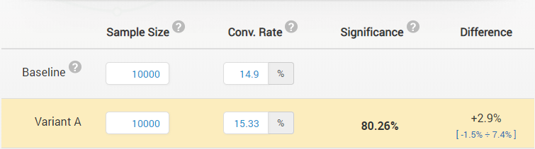
The second part of the question is more difficult to answer so I have to refer to our A/B testing ROI calculator. With a neutral prior and assuming none of the two e-mails is offering something that erodes our bottom-line, such as a coupon, free add-on, etc. more than the other, we see that an A/B test with optimal risk vs. reward ratio is one with 10,000 users per group and a significance level of 90% (p < 0.1).

Since 80.26% is less than 90% (0.1974 > 0.1 in terms of p-values) we would be risking too much in going with variant B so we should stick to our control A. The 90% one-sided relative difference confidence interval spans from -1.5% to infinity and thus we can not exclude with 90% probability the potential for B to be, in fact, inferior to A.

How to achieve higher certainty

I’m sure some of you are wondering how to get higher certainty for the decisions you intend to make. Before covering that I would like to make it clear that there is no way to have 100% certainty. No matter how big an e-mail list you have, there will always be a tiny probability of error. Even if you observe a statistical significance of 99.999% (p = 0.00001) there is always the possibility that you simply observed a very rare outcome or that some test assumptions were not met for some reason (the statistical model does not reflect reality).

That said, there are two ways to get higher certainty: test with larger numbers of email recipients or test more dramatic changes. You need to either increase the number of data points, or you need to reduce the signal to noise ratio (event rate vs. non-event rate). Both of these are ways to either get higher certainty, or to conduct more sensitive tests with the same level of confidence (more on that in “Statistical power” below).

While early on coming up with dramatic changes that are true improvements is relatively easy it becomes progressively hard after you’ve improved template, copy, subject line, etc. multiple times over the course of years. In fact, it becomes both more likely to test inferior options and to test variants which are significantly (in magnitude) worse than your current best. This is a manifestation of the well-known economic law of diminishing marginal returns.

If you have reached that point, then increasing the number of recipients you test with becomes the main option to get higher certainty. However, this is now riskier since you are losing money with each test e-mail you send out that is worse than your current best. I’ve discussed this and other trade-offs in significant detail here and here and the A/B test ROI calculator I’ve devised is a way of making statistical designs that achieve optimal balance between risk and reward.

Another approach is available when testing templates, landing pages, and other elements that persist from e-mail to e-mail, as well as more general hypotheses like “shorter subject lines work better”. What I propose is to randomize at the recipient level and then consistently send out the same template, landing page type, subject line type, etc. to each of the two or more groups. The sample size for the groups will be fixed at the beginning (contacts acquired after the test has started will not participate), as well as the time at which you will analyze the data, say 12 weeks from now. This will make any real effect more pronounced and it will also allow time for any novelty effects to wear off and any learning effects to kick in, resulting in a better long-term prediction.

Obviously the KPIs for such “delayed measurement” tests need to be recipient-based, not e-mail based. Performance metrics like purchase rate per recipient, lead conversion rate per recipient, proportion of recipients who opened at least one email / clicked at least one email will be easy to work with statistically, while metrics like average revenue per recipient, average e-mails opened per recipient, and average e-mail clicks / site visits per recipient will be useful as well, but their non-binomial nature should be taken into account.

Statistical power (but what if variant B is truly better?)

Continuing with the above example one could say: but what if variant B is truly better than A? After all, such an outcome would have only been observed with probability 1 in 5 if that was not the case. They will be right to ask that as it is in fact, a possibility.

Just because we did not observe a high statistical significance (low p-value) does not mean the tested variant is not superior to the control. One statistical concept that can answer the above question is that of statistical power which is defined as the probability of observing a statistically significant outcome when a true difference of a given magnitude is present. It is mostly important during the statistical design phase.

In planning the e-mail A/B test so as to expose 20,000 users in total to our variant and control we have 80% probability of detecting a true relative improvement of about 10.32% (CTR improving from 15.00% to 16.55%) and even higher power to detect larger possible true improvements. Knowing this in advance can inform our decision whether to test or not. If there is very low chance that our changes result in a true improvement of this magnitude we would need to reconsider the statistical design. In this case the numbers were arrived at using the ROI calculator so they are optimal and running the test is justified given our input parameters, however in other cases it might not be.

In short, statistical power is useful pre-test to understand how big a difference we can detect reliably, what the sensitivity of our procedure is. After the test, since we did not observe a statistically significant outcome while having 80% or higher probability of observing one if the true effect was 10.32% or higher, we can, with 80% probability, rule out true improvements higher than 10.32%.

However, after the data is gathered it is more informative to examine the one-sided confidence interval with our chosen significance threshold. In this case the 90% interval spans from minus infinity to 7.4%, confirming that with 90% probability the true magnitude of the difference is below 7.4% (or, more technically, that a confidence interval constructed using the same procedure would contain the true value 90% of the time).

Sequential statistical methods for efficient e-mail A/B testing

As already pointed out, using fixed-sample tests restricts us from “peeking” at the data and making decisions as we gather more information. Having to make a decision about a test’s sample size and minimum detectable effect in advance is sub-optimal in the many cases when the true effect is either significantly positive or significantly negative than the minimum detectable effect for which the test was planned.

Using a fixed-sample test means that even if a test is looking very promising or abysmally bad, we can’t stop it without compromising the statistical error estimates. Even just a couple of peeks at the data with intent to stop can result in the actual error being several times higher than the nominal one we will get if we calculate statistical significance or confidence intervals without accounting for the peeking. A deeper explanation and more on the effects of peeking can be read here.

So, how do we maintain the ability to examine the test data as it gathers while retaining statistical guarantees? By using sequential methods developed specifically for that purpose.

Sequential methods for statistical analysis still require the specification of things like the expected baseline conversion rate, the minimum effect of interest (or minimum detectable effect, MDE), significance level and power. On top of that one needs to estimate roughly how many times they expect to look at the data.

With e-mails it should be relatively easy to do. For example, if a ROI-optimal design for testing open rate calls for 48,000 e-mails to be sent out in order to reach an optimal level of statistical power. You can take a look at your current e-mail list size (~8,000 strong) and expected growth rate and determine that you will need to send out 6 e-mails to your list in order to reach this number of e-mails.

It makes sense to look at performance after each e-mail is sent out, and not in-between, and so you have 6 times at which you would like to examine the data and be able to call the test, if the results are conclusive enough. Each time you’d have data from 8,000 more e-mails to work with.

With this information at hand, efficacy and futility boundaries can be constructed that will provide guidance on whether to stop the test in favor of one of the variants or to continue testing until more reliable estimates can be achieved. This also why these are often called “decision boundaries”.

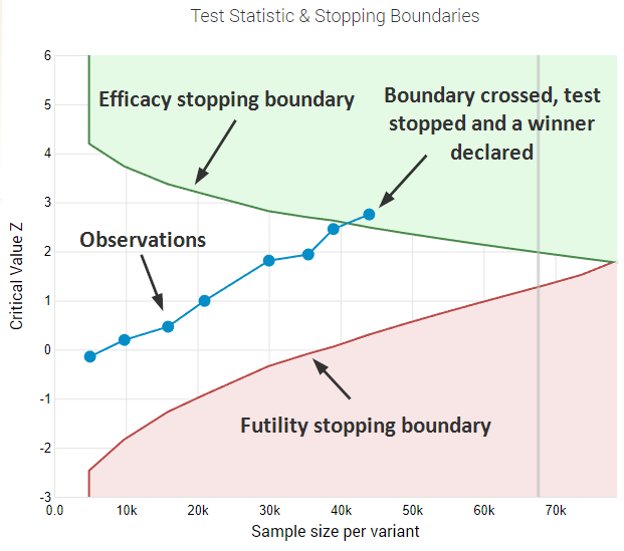
The result from applying the boundaries is a marked decrease in the average sample size (number of recipients/subscribers/contacts, users) you need to maintain the same power with the selected significance threshold:

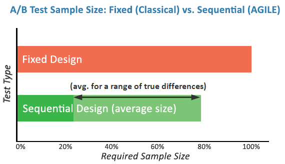
Sequential tests can also be employed for single e-mail burst tests given proper technical capabilities. For example, the Black Friday e-mail campaign above can have its MDE reduced from 10.32% to 7.25% while improving the risk/reward ratio from 1/13.69 to 1/28.37 (2x improvement) by testing with 20,000 recipients in the test at the worst case but with a high probability of stopping the test much earlier if the results are overly positive or negative (8 equally-spaced looks, each after sending out 2,500 e-mails).

A/B vs MVT (A/B/n) tests

While I have restricted the discussions above to A/B tests, everything above applies equally to A/B/n tests, often called multivariate tests (MVT). However, one should understand that statistical adjustments are needed when testing more than one variant versus the control with the most powerful procedure being the Dunnett’s post-hoc test. If no adjustment is applied, then the probability of observing a false positive increases significantly with each variant added to the test.

To maintain the same power relative to the same minimum detectable effect the overall sample size needs to be increased, but the sample size per group actually decreases. Note that many sample size calculators do not support or incorrectly calculate sample sizes for MVTs, and similarly I’ve seen cases where no adjustment is made, or inefficient adjustments like Bonferroni are used instead. I can guarantee that our own statistical calculators do not suffer from such issues, but you’d need to ask your vendor if you are using different tools.

In general, this should not be a turn-off, especially if there are well-thought out competing variants which differ significantly between each other. It should be noted that in general such tests are powered to detect significant differences between the control and the variants but would lack sensitivity for the usually smaller differences between the variants.

It should be noted that testing poorly thought-out variants just for the sake of it will likely result in loss of revenue during testing, with little chance for recouping the testing costs due to detecting a true improvement.

The usual inferential caveats apply

The usual warning about applying what was learned from a sample to a whole population hold, mainly that for this process to be valid the sample should be representative of the population. Transferring what was learned from tests on Black Friday, Christmas or New Years to the rest of the year might not be valid.

Similarly, testing during the summer months may yield conclusions that are specific to summer campaigns when people are checking their e-mails while on vacation and these may not apply or even be reversed for the rest of the year. What works in the UK may not work in the US or Australia and vice versa.

Also, things change. What worked 10 years ago may no longer work due to external changes like changing technological landscape, economic factors, competitor practices, regulatory interventions, etc. These are all examples of unmeasurable risks and statistical significance calculation from your usual A/B test cannot capture them. Underestimating these unmeasurable risks is not recommended.

I hope this was a useful introduction to the statistical approaches one can use in A/B testing in email marketing. No matter if you are optimizing open rate, click-through rate, conversion rate or revenue per recipient, you should be off in the right direction if you follow the advice above.

About the author