The A/B Testing Guide to Surviving on a Deserted Island

The secluded and isolated deserted island setting has been used as the stage for many hypothetical explanations in economics and philosophy with the scarcity of things that can be developed as resources being a central feature. Scarcity and the need to keep risk low while aiming to improve one’s situation is what make it a good setting for this story in which I attempt to demonstrate the A/B testing approach of managing risk.

This story will help you get a glimpse of the complexities involved, of some of the methods used to address them as well as the limits of learning about and predicting people’s behavior through experimental methods. If you are already familiar with A/B testing I hope you will find the post a somewhat entertaining overview with maybe a thing or two you can add to your existing knowledge. If you are a newcomer to the field I hope the exposition is not too dense and I encourage you to follow the references for a more detailed understanding of what is presented.

A statistician gets stranded on a desert island…

This is how our story starts. A statistician and his fellow colleagues become stranded on a small uninhabited island like this one:

The particulars are unknown, but we can speculate that it was because of their constant pointing out to higher ups that no set of observational data, correlations and regression analyzes can prove a causal link. Or maybe it was their insistence on the need to take the egression from the mean effect (opposite to regression to the mean) into account when estimating the yearly bonuses based on observed performance.

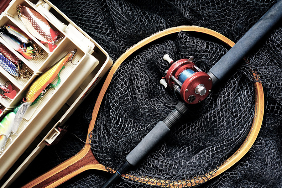
Regardless, the result is that now the apex predator has to survive as a fisherman as the only thing the group has available is a set of fishing rods and some baits. They are currently capturing 20 fishes per day securing them 10 kg of fish meat total (about 0.5 kg of meat each), on average. This is barely able to sustain them, so they need to increase that amount in the most risk-free way possible.

This need is also due to the fact that a reserve for bad days needs to be maintained for when he is ill or incapable of fishing for other reasons such as bad weather, etc. The current reserve food available is equivalent to 105 fishes (52.5 kg of meat). This means, for example, that capturing less than 7.5kg of fish per day on average for over 3 weeks will deplete the reserve and our statistician turned fisherman and his friends will die of starvation.

Obviously, the above can be satisfied by capturing more fish, by capturing larger fish on average, or by doing a combination of both.

We know that these 20 fishes caught per day constitute 1% of the fish around the island in any given day. Captured fish is replenished by the beginning of the following day so that the total number of possible fishes to catch remains around 2000 fish per day. Some of the fish may come around the island several days in a row, or after skipping a few days, while others may only be encountered once and never seen again, perhaps due to them ending up in the belly of a predator fish.

Our fisherman can experiment with different fishing locations, different equipment, and different baits, as well as different times of the day. Furthermore, they know that in these seas fish are abundant except for the winter months when they are less active. It is also known that through some peculiar effect past Christian missionary efforts resulted in the fish behaving somewhat differently on weekends compared to workdays.

If we are to lay the circumstances briefly, we have:

Goals: need to increase food reserves (dried fish meat) while minimizing the risk of dying of starvation and utilizing his limited resources as efficiently as possible.

Risks: reducing their fish consumption to fewer than 7.5kg per day (0.75% of available fish) for over 3 weeks for any reason will result in a lethal outcome for the whole group.

Rewards: capturing more fish, resulting in more leeway and better reserves for (literally) rainy days, sick days, etc.

The superpower of Randomization

Because what is a good statistics story without a superpower? Other than his command of statistical methods and design of experiments our statistician has the unusual ability to be able to randomly select fish that will be directed towards a chosen rod and bait. In other words, his superpower is randomization. Conveniently, this allows him to model any unknown or unmeasured factors as random variables, allowing for randomized controlled experiments and statistical analyzes of their outcomes.

Survival Task 1: Identify what you can and can’t measure. Choose Key Performance Indicator(s).

Measured outcomes: The group agrees that they can accurately measure the number of fishes caught and their weight and that these are sufficient measures assuming nutritional content does not markedly differ.

Measured factors: The group can observe atmospheric weather (sunny, rainy, cloudy, windy, stormy, approximate temperature) and water temperature with some degree of accuracy. There are also the 4 sides of the island on which one can fish, with a total of 8 bays (2 on each side).

Unmeasured factors: The group cannot know in any detail the local and global water currents or how predatory fish & other fish migration patterns are affecting the fish population around the island. They also cannot appreciate minute differences in bait quality and cord thickness, water aeration changes, and infinitely many other such influences.

Based on the above, the hero of our story decides to record what can be measured in terms of outcomes and factors and to conduct a randomized controlled experiment in order to be able to model the unmeasured confounding factors as random variables and thus elicit a causal link between whatever attempt is made at improving fish yield and the outcome.

The benefit of conducting an experiment versus simply making and using new equipment or bait and observing the outcomes is that the group would be able to estimate the probability of being tricked in thinking they are better than or worse than their prior equipment in securing fish. Changes in the environment, fish behavior, predator prevalence, water currents and other unknown factors that could unknowingly bias any comparison of post- versus pre- data would not affect the outcome of a proper experiment. Even better, through the experiment the group will obtain an unbiased estimate of the increase or decrease in yield that the new equipment is providing them.

Survival Task 2: Calculate risks vs reward ratios, choose experimental & statistical design

Test idea #1: Better fishing gear

The first idea that our poor statistician considers is that they can invest time and resources in making a stronger rod and weaving a thinner and stronger cord. The idea is that it will allow him to capture bigger fish (whereas before the cord would snap or the rod would break) and that the thinner cord also makes it easier to fool fish into taking the bait.

Our poor stranded fisherman could only wish he had equipment like the one above!

It will cost the group 20 fishes of energy from their reserve to produce the improved rod and cord for testing on top of the energy they would have expended on making a replacement rod and cord of the current type. It will also cost them 20 more fishes per month in spending time producing the stronger, better rod and cord, despite it being a bit more durable. They cannot risk a decreased fish yield for too long as it will affect future survival chances.

Our fisherman has some idea about the better performance of the stronger rod and cord in capturing bigger fisher that are otherwise able to escape: about 10% of all fish. So, on average, he expects to be able to catch about 11% more fish in number and even more in terms of meat weight. However, this might be offset by unknown effects on the rest of his fishing, so, having no good data to support his assertion he decides to reduce his expectation to about 5% and thus his prior is normally-distributed, centered on 5% relative increase with a fairly large standard deviation of 15% relative change (variance = 0.8 sd):

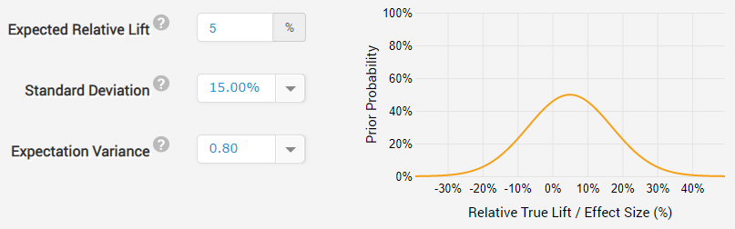
With such a prior the statistician is basically saying that due to prior experience of fish breaking away free he expects the new gear he introduces to result in an increase in the quantity of captured fish but allows for a decent probability that it might reduce it significantly as well due to unexpected effects. There is also some probability that he underestimated the amount of improvement that can be achieved with the new fishing equipment.

Assuming they might be on an island for a long time and that it is unlikely to experiment with the strength of the rod and cord anytime soon, a 5-year period during which they expect to benefit (or suffer) from adopting the new fishing gear is reasonable.

As they have no control over the overall amount of fish present, and thus: the absolute number of fishes caught, the group decides to focus on increasing the percentage of fishes caught, while keeping an eye on the weight of the fish. The percentage caught is a binomial metric which can be modeled using the binomial distribution for which the standard deviation is known and does not require estimation. Since there is little doubt that the fish that will be caught with the new fishing equipment will be, on average, larger in size, there is no need to do these calculations for the non-binomial metric of average daily meat yield. If it were not the case, this would somewhat complicate the statistical calculations and increase the length of the fish gear experiment. The tests used will obviously be one-tailed (one-sided hypotheses) since we are interested in both the size and the direction of the effects.

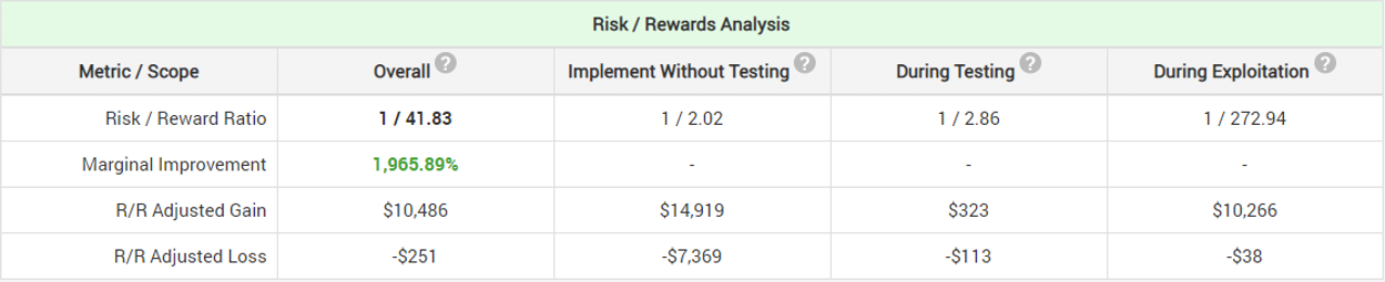
With all the above considerations the risk-reward calculation reveals that by using a simple fixed-sample procedure in which they only gather once to evaluate the results of the experiment and decide whether to use the new fishing equipment or not, the optimum level of risk of adopting the new fishing gear if it is in fact no better or worse than the existing one is 9% (91% significance threshold) and a test duration of 8 weeks which has 80% statistical power for detecting a true improvement of 13.40% (relative). This means that if the true improvement is smaller it will be less than 80% likely to be detected with a statistically significant outcome.

(click on any image in the post to view it in full size)

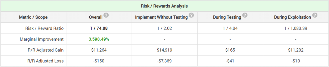
By using this design our statistician is able to estimate that he will achieve a 20 times improvement in his marginal risk-reward ratio. If they were to just start using the new equipment without any testing whatsoever, even if his prior assumption about the possible effect is correct they have a risk/reward ratio of 1/2.02, meaning that they can achieve an increase in the number of fish caught over the 5 year period by 150 kg (300 fishes), however they might also decrease their yield by 74 kg (148 fishes) (probability-adjusted numbers, min and max are much higher). By testing, this ratio improves 20x to 1/41.83. The maximum probability-adjusted gain was estimated to be a good 779 kg of fish over the 5-year period (1558 fishes) while the maximum probability-adjusted loss is only 13 kg (26 fishes).

Evaluating the outcomes as you go?

At this point, however, a member of the group points out that if the new fishing equipment is in fact performing significantly worse than expected or if there is little chance to demonstrate efficacy, it makes sense to cut the experiment short, otherwise it will unnecessarily diminish their food reserves. Also, if the performance is so much better than expected, it would make no sense to continue using the old equipment for the entire duration of the test. The suggestion is to count and weigh the fish at the end of each day, add them to all the prior counts since the beginning of the experiment and see if there is a statistically significant difference. If there is, the test will be stopped, and the winning equipment adopted for use.

The statistician, however, understands the assumptions behind the statistical significance calculation method and vehemently disagrees as peeking at the data and recalculating significance on a daily basis with intent to stop the experiment will actually bias the outcome and ruin the validity of the statistical estimates. He explains that if a test has been monitored and a statistically significant outcome was not obtained on days 1-6, but one was obtained on day 7, then it is less of a proof for a true effect than if it had been not monitored in days 1-6 and only checked on day 7, since the former test has failed more chances to produce a significant result than the latter.

The statistician turned fisherman then explains that due to known in-week fluctuations in the behavior of fish it is best to evaluate the experiment results only at 7-day intervals, thus capturing a full week between each two data evaluations, eliminating the effect of the fluctuations.

He initially considers a simple sequential probability ratio test (SPRT), but then remembers that not only should the result of the experiment be statistically valid, but it must also be as representative of the whole fish population and of their behavior through the different cycles in time, as possible. It should also account for any novelty and learning effects. For example, initially the fish might be scared of the new unfamiliar equipment, driving yields down, while after a week or two they may become accustomed and yields can surpass the original ones. On the other hand, if the devise is unfamiliar it might initially draw more curious fish towards it, increasing the yield initially, but later flattening out or even decreasing.

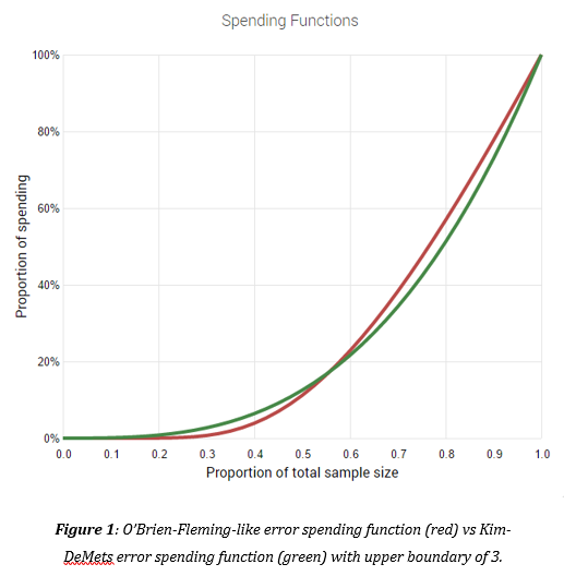
To strike a balance between the need for a faster conclusion of the test and the need to obtain a representative sample to improve the generalizability of the results, the statistician decides to use an alpha-spending function with a convex curve, meaning that it is conservative early on and more aggressive towards the middle phase of the experiment.

He recalculates the risk-reward ratio with the new sequential monitoring approach in which yields are analyzed every 7 days and significance calculations are compared to an efficacy and futility boundary to decide whether to stop prematurely and start using the new equipment or drop the test and stick with the current one.

The calculations reveal that for optimal improvement in the risk-reward ratio the experiment should now be planned for 18 weeks (expected duration is 5 weeks vs 8 weeks for the fixed-sample design) and a significance threshold of 94% (vs 91%). The test now has 80% power at 9.74% relative effect (vs 13.40%).

As expected, the implementation of a sequential evaluation scheme significantly decreases the average expected duration of the test, as well as improves its sensitivity to smaller true effects. The resulting marginal improvement in the risk-reward ratio reflects that as it is now 36x (vs 20x with the previous approach), which is a significant increase in the likelihood that they will accurately evaluate the new fishing equipment without an undue increase in their risk exposure. The maximum probability-adjusted gain was estimated to be a whopping 855 kg of fish over the 5-year period (1710 fishes) while the maximum probability-adjusted loss is only 15 kg (30 fishes).

A/B or A/B/n?

Almost ready to relax after thinking that his work is done, our statistician starts to consider that maybe the stronger and thicker rod’s larger shadow may scare some of the fish away, while the thinner cord in itself might be a major improvement, even with the current flimsy rod. This means that a combined experiment with a stronger rod and better cord in one test variant will not be able to reveal the reason for any improvement and in fact may obscure the positive effect of one of the two proposed changes.

Since our group of survivors is mainly interested in the combined effect of the equipment changes with the individual contribution of the rod and the cord being secondary considerations a factorial design is inappropriate but running a multivariate split test (MVT a.k.a. A/B/n test) makes sense.

Therefore, it is decided that the experiment will instead be split into four test groups: one control, one with stronger rod and regular cord, one with thinner cord and regular rod, and one with stronger rod and thinner cord (denoted control, A, B, and C).

Since only one set of equipment will be chosen at the end, the statistician knows that he needs to account for the error rate of this set of pairwise claims (A > control, B > control, C > control). If the error rate for each comparison is set at the desired 6% level (94% significance threshold), the overall error rate for all three comparisons will surely be significantly higher than that: approximately 17% (1-(1-0.06)^3) instead of 6%, assuming they are not dependent.

Since these are three treatments compared to a common control, there is bound to be dependency in the results therefore the classic Bonferroni correction (0.06/3 threshold for each comparison) will be too conservative, unnecessarily reducing the sensitivity of the experiment and making it less likely to detect a true improvement in efficiency, if it exists.

A more powerful procedure in this case is Dunnett’s Step-Down method. Luckily, the statistician finds in his backpack a set of Dunnett’s correction tables and is able to use them to calculate the required sample size and later: the required adjustments to the p-values from the pairwise comparisons.

After accounting for the doubling of the cost of the A/B/n test compared to the previously imagined A/B test (needs to prepare two strong rods and two thinner and stronger cords instead of one of each), the recalculated risk-reward ratios reveal an approximately optimal maximum test duration of 30 weeks (expected duration of 9 weeks) and 90% significance threshold giving the test 80% sensitivity to a true effect of 8.32%.

While the multivariate test has worse risk-reward ratio than the A/B test (1/45.63 vs 1/74.88) the stranded group decides that it is worth conducting it as it provides more detailed information and testing more equipment combinations at the same time. It also removes the probability of missing out on a possible improvement due to contradictory effects.

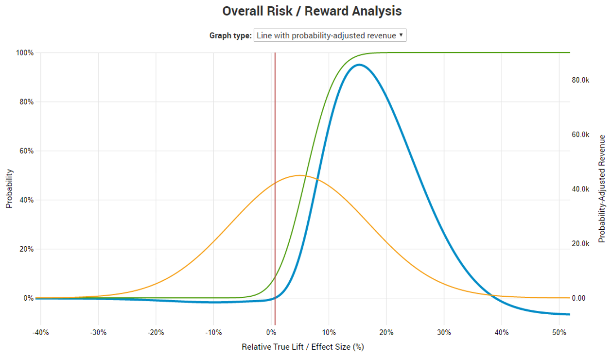
Due to the low testing cost and relatively low maintenance cost the probability-adjusted break-even point is a mere ~0.6% relative lift. However, had the break-even point been higher, a different analysis would have been needed in which the null hypothesis is not that of no or negative difference, but one of less than 0.6% improvement.

Test idea #2: Different bait

A similar vain of thoughts and considerations was applied to the idea of experiment with different bait, nothing the increased threat to the external validity of the outcomes in case the fish population changes due to seasonal migrations a myriad of other factors. It was considered a more fish-type-sensitive approach needs to be used wherein results will be analyzed on the segment level: each bait’s efficacy will be evaluated for each of the four fishing locations as they feature different types of fish. If the fish in one location responds better to one of the baits, it can easily be targeted with that bait only.

As there weren’t an abundance of options only two types of bait were considered: one control (A) and a test variant (B). A mixture of the two was not considered at this time.

Since some interaction effects between the types of bait and the fishing equipment used were expected, the two experiments would be conducted concurrently, on the same fish population, but the results will be analyzed for strong and opposite in sign interactions to avoid the danger of choosing the bait based on improved performance of that bait with the old fishing equipment while it does worse with the new one (which might be chosen after the first experiment is completed).

Siloing of the experimental groups wherein a proportion of the fish will be exposed to only the first experiment while the rest of the fish would be exposed only to the second experiment is rightfully rejected as it is both less efficient and allows for interactions to be adopted without any test whatsoever, defeating the purpose of testing.

Task 3: Conduct the experiments, analyze the data

Test #1: Better fishing gear

The group prepared the new equipment and started the experiments. Analyzing the data after week 1, they see these results for the first test:

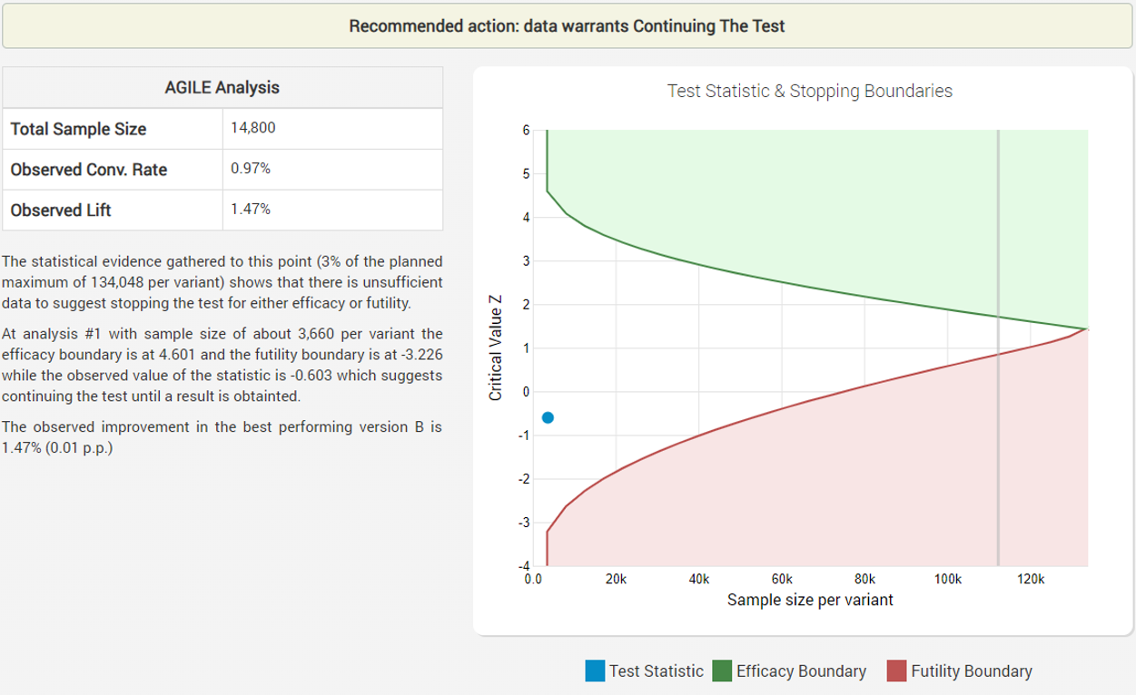
Despite the early negative results, the futility boundary has not been reached so the fisherman continues to observe the data on a weekly basis until at week 5 the adjusted statistic finally broke positive territory:

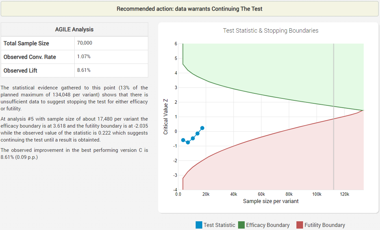
The experiments continues and at week 12 it concludes with a success, stopping after only 37% of the expected duration if a fixed sample size test with the same parameters (significance level, power and MDE) was conducted:

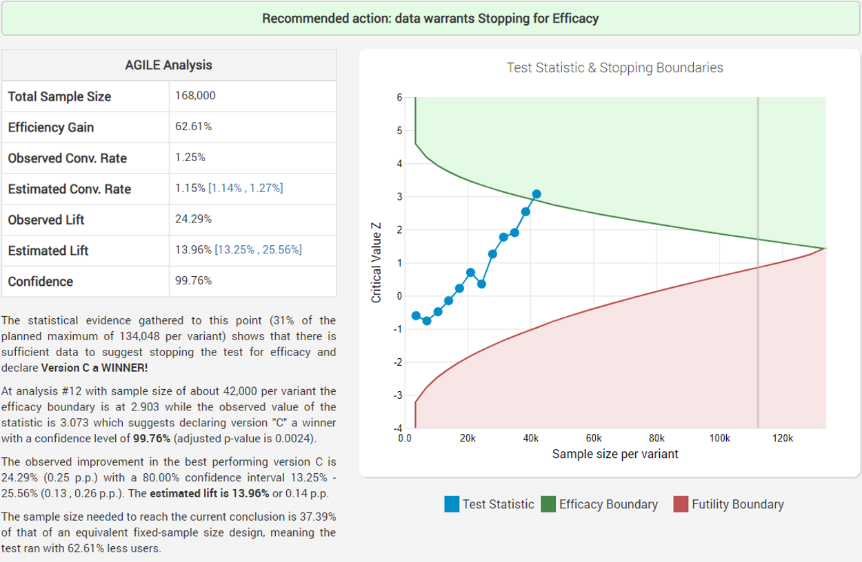
While the observed improvement in the number of fishes caught is just above 24%, the bias-corrected estimated lift is 13.96% with a 90% one-sided confidence interval bound of 13.25% which is way above the minimum impact necessary to justify the new equipment (~0.6%).

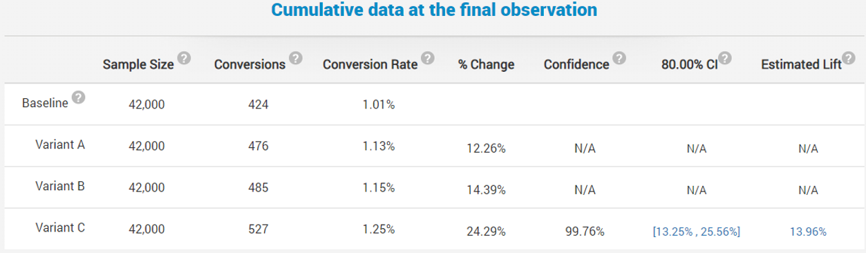
The data shows that both Variant A and Variant B show some improvement, although not as impressive as the variant in which both the rod and the cord were changed (C).

With such conclusive results the group was certain that going forward they will be catching more fish than they previously did if they start using the new fishing gear. This can be inferred since if the new gear was performing equal to or worse than their existing one such a rare outcome would be very unlikely (strong argument from coincidence). Still, they would need to continuously monitor the fish population for major changes that may put the validity of the results into question and require a re-test.

While the experiment cost them a few weeks of suboptimal fishing, it was a good trade-off given the risk of starvation if the new gear actually had a detrimental effect on their fish yields for whatever reason. Now even if in the future there is a downtrend in the total quantity of fish caught, they’d be fairly certain that it is not due to the gear in their hand, unless they were also observing a significant change in the overall composition and behavior of the fish population: qualitatively different types of fish they haven’t seen before, etc. in which case a reassessment might be warranted.

As there were no significant differences in performance found between the different fishing locations and weather conditions, no further consideration of these segments was necessary.

Test #2: Different baits

The test with the two different baits ended a week before the fishing gear test with the following outcome:

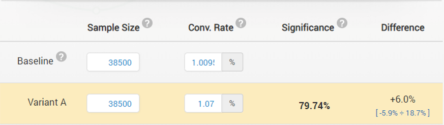
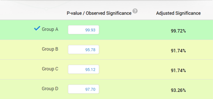
With a significance threshold of 95% the tested bait obviously failed to demonstrate its overall effectiveness. However, upon analysis of the outcomes by fishing location it turned out that it is in fact significantly better in all but one of the 4 sides of the island (consequently in all but 2 of the fishing locations):

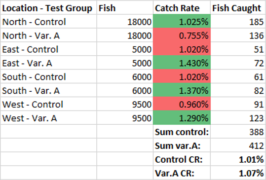
Not only that, but the outcomes for the new bait in the East, South and West location are statistically significantly better than those of the old bait, making it a mild example of the Simpson’s paradox. While seeing one statistically significant outcome is fairly probable (~19%) even if the bait actually performed the same at all locations, this question is irrelevant since we are looking to make individual decisions for each site (to the same effect we could have instead performed separate tests, which is recommended when there is reason to suspect significant differences due to efficiency gains due to different MDEs and/or using a sequential monitoring method). This situation is different than multiple testing issues that arise when working with more than one performance indicator which would require multiple comparison adjustments in all practical cases.

If one is nevertheless worried about rejecting the overall hypothesis that there are no differences at any of the sites, effectively controlling the rate of tests with at least one statistically significant segment, multiple testing adjustments would result in the following adjusted values:

The North comparison is actually decidedly against Var.A (95%CI_upper = -12%) so we can be quite certain that it will have detrimental effects there.

While we do not know what is causing this: whether it’s the type of fish, the type of water, water currents, etc. we can be fairly sure that if we are to use the bait from Var.A in the East, South and West and our old bait in the North, we are going to see a significant increase in our average yield (95%CI_lower = 16.2% lift). Since we are in fact changing the bait in 3 out of 4 locations, here is the combined comparison between the two types of baits at locations East, South and West:

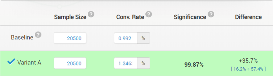
The statistical significance of this claim is, expectedly, also very high. The decision was made to use the bait from Var.A when fishing on the East, South and West sides of the island while the control bait continues to be used on the North side. Not that all significance calculations and confidence intervals for Test #2 were calculated for the actual percentage change (% lift), and not naive extrapolations from absolute change statistics.

There were no differences when segmenting the data by weather conditions: both baits did about equally in the major types of atmospheric and water conditions. While the test was not powered to detect smaller differences in those subsegments and our “no difference” conclusion is weak, we also do not have the data to suggest using one of the baits when certain weather conditions are present.

And they lived happily ever after

While there are no guarantees for that, but assuming they weren’t witnessing extremely rare coincidences they should be just fine.

This is where we leave our stranded statistician and his friends – waiting for a ship to rescue them, but at least they have bellies full of tasty fish. They surely were happy with their initial ideas for improving their survival chances, same as many A/B testing programs are hitting improvement after improvement in the early stages, especially if the baseline is not so great and opportunities to improve abound. They are surely also happy that they minimized the risk of things going quite badly for them, either in terms of missed opportunities to choose a better set of gear or in terms of starving to death without really knowing why. The inevitable cost of risk reduction, while being very real, is much lower than the losses protected against.

Was the above presentation useful? Did it help you understand A/B testing as an outsider to the field? If an insider, did it create a more cohesive picture in your mind, or point out things that you did not appreciate enough before? Leave a comment to let me know!

All calculations in the article used our statistical tools: the sequential A/B testing calculator, the A/B testing ROI calculator, and the basic statistical calculators.

About the author