I got a question today about our AGILE A/B testing calculator and the statistics behind it and realized that I’m yet to write a dedicated post explaining the efficiency gains from using the method in more detail. This despite the fact that these speed gains are clearly communicated and verified through simulation results presented in our AGILE statistical method white paper [1].
In this post I’ll present simulation results of the efficiency of using AGILE for statistical analysis of A/B tests, a.k.a. online controlled experiments and shows that (spoiler!) yes, it does result in 20-80% faster tests, on average, with a small trade-off involved.
A/B test duration – Simulation setup
The improvement in test duration one can get with the AGILE A/B testing method is measured against a fixed sample size test with the same basic parameters due to the following reasons:
- fixed sample size significance tests are the norm in most CRO books, blog posts and advice in general
- fixed sample size tests are easiest to understand and plan
- it is a standard comparison to make, so indirect comparison to other tools and approaches is possible using their own comparisons to fixed sample size tests
- comparing to other vendors is difficult due to proprietary technology and much higher testing costs, if automated testing is even possible.
The setup of the simulations is as follows: an A/B test with one control and one variant (A), the null hypothesis being that there is no or negative difference between the variant and the control, while the alternative hypothesis is that variant A is performing better than the control. Thus, both hypotheses are composite, just as in most real-life scenarios.
If you wonder why a one-sided hypothesis is used instead of a two-tailed one, check out One-tailed vs Two-tailed Tests of Significance in A/B Testing. The alternative hypothesis is a superiority one, but the simulation results are generalizable to the non-inferiority case as well.
To verify the whole AGILE A/B testing statistical method, a series of simulations was performed with a set of true values for the conversion rate of the variant tested. If we denote the minimum effect size (lift) of interest (MDE) as δ (delta), the true values for the alternative hypothesis (variant A conversion rate) were spread as -1⋅δ, -0.5⋅δ, 0⋅δ, 0.5⋅δ, 1⋅δ, 1.5⋅δ, 2⋅δ, covering positive, negative and zero true differences. The control is thus at 0⋅δ. Random numbers were then drawn from a Bernoulli distribution using the rbinom function of the R software around each true value – 10,000 simulations for each, totaling 70,000 simulation runs. A random seed was set on each simulation run.
The design parameters were α = 0.05, β = 0.1, the minimum relative improvement of interest at 15%, the baseline at 5.0% conversion rate. The number of statistical analyses set to 12, simulating a typical test running for 12 weeks = 3 months. A non-binding futility boundary with disjunctive power was used – the latter not being important in this case as the A/B test in question has just one test variant. This corresponds to 5% false positive error threshold and 10% false negative error threshold.
We chose the error thresholds to be typical, but the results are generalizable across the whole range of valid values for alpha and beta. I strongly encourage CRO professionals to use our A/B Testing ROI calculator or another solution to the issue of balancing risk and reward from A/B tests when deciding on the errors they are willing to accept in both directions order to test in reasonable time frames.
Simulation results: Speed gains & Trade-offs
This is directly copied from Figure 14 of the white paper and presents a comparison between a classical fixed sample size significance test of the same parameters (significance threshold α, power β, MDE δ) as the AGILE A/B test. The true lift of variant A is given in relative percentages as well is in terms of δ for convenience. The average stopping stage is calculated using the arithmetic mean.
|
True Variant A Lift |
Average Stopping Stage (12 max) |
% of Tests Stopped After the Fixed Sample Size |
| -15% (-1⋅δ) | 2.87 | 0.00% |
| -7.5% (-0.5⋅δ) | 3.99 | 0.18% |
| 0% (0⋅δ) | 6.22 | 6.99% |
| 7.5% (0.5⋅δ) | 8.26 | 23.14% |
| 15% (1⋅δ) | 7.27 | 11.37% |
| 22.5% (1.5⋅δ) | 5.23 | 0.84% |
| 30% (2⋅δ) | 3.84 | 0.01% |
Looking at the percentage of tests stopped after the fixed sample size it becomes clear that an AGILE test is more efficient, on average, than a fixed sample size test for all cases examined, but there are still individual tests where an AGILE test will take more users to complete than a fixed sample size test. This is the price one pays for the average efficiency gain and for the flexibility of interim analysis. The percentage of tests that end with more users than an equivalent fixed sample size test is very small, even at extreme values, as seen in the third column in the table above – 23% in the worst case of about ~0.5⋅δ, and progressively less as the true difference between the variants gets smaller or larger than that. If the true difference is 1.5x larger than the planned MDE, then a fixed sample size will be slightly more efficient in less than ~1% of cases. If the result is 0.5x MDE in the negative direction, only ~0.2% of fixed sample size tests would be more efficient than AGILE.
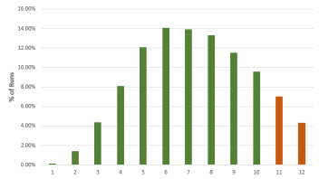
The average stopping stage gives us an idea of how much faster an AGILE test is. In this scenario stopping at stage 11 or 12 will put us past the fixed sample size, as shown below:
(click image for full size)
Since all values are, on average, smaller than 11 in all cases, AGILE is, on average, more efficient for all possible true differences.
See this in action
The all-in-one A/B testing statistics solution
While the average stopping stage gives a good idea of just how much more efficient an AGILE test is versus a fixed-sample size counterpart. However, as we all know, averages can be deceiving, so here is a detailed breakdown for each of the true differences in the above table, with green bars for cases where the sample size is less than the fixed-sample size, and dark orange where it exceeds that of the fixed sample size test counterpart:
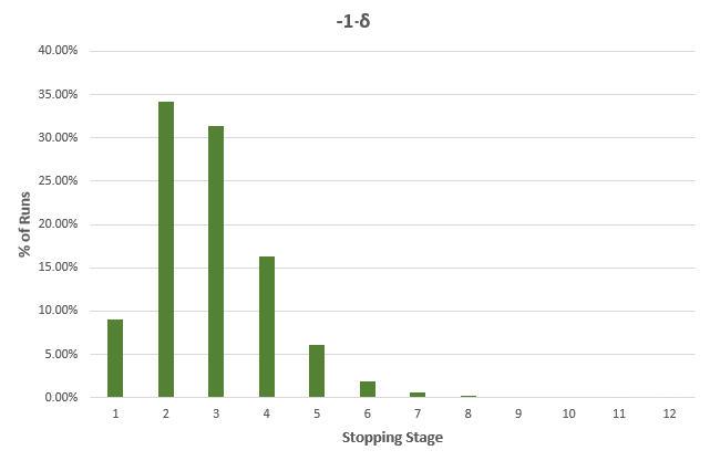
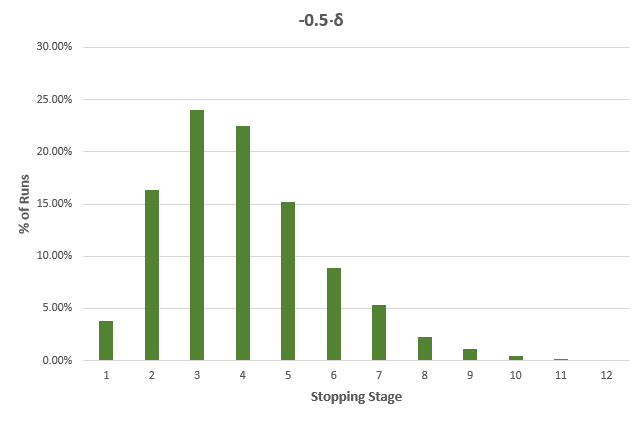
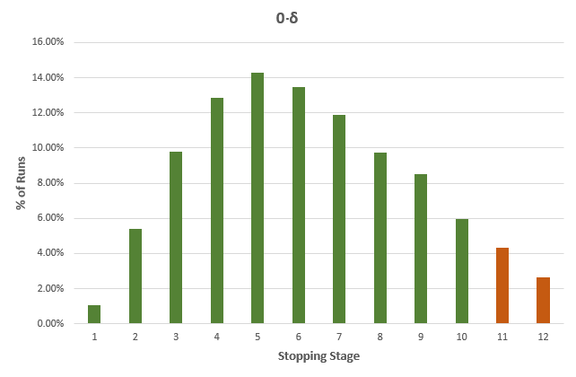
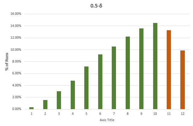
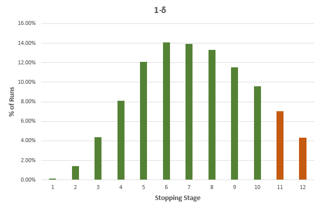
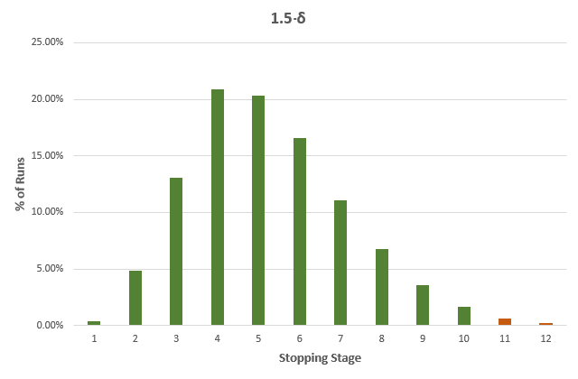
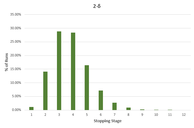 It is evident that the larger the true difference is, in either direction, the faster an AGILE A/B test will be compared to an equivalent fixed sample size test.
The results are mostly generalizable across a large range of test parameters with MDE and baseline conversion rate playing no role, while altering the number of analyses has a pronounced effect: reducing the number of analyses reduces the effectiveness of AGILE, e.g. an AGILE test with 6 analyses has less opportunities to stop early for either efficacy or futility, and is thus less likely to be more efficient, and a test with just one interim analysis will be least efficient. For more than 12 analyses the increase in effectiveness is negligible for most practical purposes, e.g. increasing the number of analysis from 12 to 20 results in only ~1% better average efficiency.
Predicting the duration of an AGILE A/B test
Now, to understand why we claim 20-80% faster A/B tests and not a fixed % improvement, one needs to understand that it is not possible to fix the duration and thus the sample size of a test with interim analysis of significance. That is one of its main advantages – we can stop at any time if the results are unexpectedly positive or negative. However, this turns into a challenge when we need to compare test durations: the fixed sample size test is, well, fixed, while the duration of the AGILE test will depend on the number of interim analyses and the true difference between control and variant.
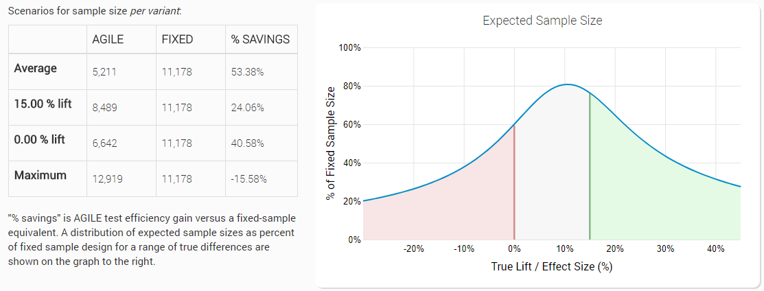
Therefore, when comparing the performance improvement, we need to consider the range of possible true values and their distribution. This is a subjective thing and furthermore – will vary from test to test – both in range and distribution, especially given that the main variable is MDE, which in itself is a somewhat subjective choice. I argue that there are ways to make that choice a much more objective one by considering the costs and benefits and risks and rewards from running an A/B test with a given set of parameters. Luckily, there is a numerical method to estimate the average sample size at different values of δ, which is something each of users sees when designing an AGILE test:
(click image for full size)
As you can see, for a range of true differences between -2⋅δ to +3⋅δ the minimum improvement in average duration is 20% at exactly 0.7⋅δ, while the maximum is 80% at -2⋅δ and this is how the best case and worst-case range of 20% to 80% improvement in speed of A/B testing is derived. Surely, one can criticize the choice of this range, but we believe it to be a good guess based on our prior experience in analyzing A/B testing data.
The average sample size shown in the image above is simply the arithmetic mean for the whole range of true values – it is just there to give an idea, as there is no way to calculate that correctly without a prior distribution. Since the range is not equally distributed around zero, it is a conservative estimate allowing for a higher probability that the true difference will be positive, and lower probability that it will be negative. If the opposite turns out to be true, the actual average will be significantly lower. From the sample size estimates, test duration / run time can be estimated using predictions for the traffic volume of the part of the website that will be tested.
Conclusions
I believe the above clearly demonstrates the benefits of using a sequential monitoring statistical approach to A/B testing, in this case the AGILE statistical method developed by me. In terms of average speed of testing it performs better than classical fixed sample size tests for all possible true differences between control and variant(s). Where there is a possibility for some AGILE tests to run longer than an equivalent fixed-sample size test, the probability for that is low and a couple of such tests would be more than compensated by the dozens of much faster tests you can expect to run in your CRO agency or freelance practice.
For an explanation of why and how these improvements come to be, I propose reading the blog posts from the AGILE A/B testing category on this blog, especially this one, and even better – the whole white paper, linked in the beginning of the post and in the references below.
References
1 Georgiev G.Z. (2017) “Efficient A/B Testing in Conversion Rate Optimization: The AGILE Statistical Method” [online] https://www.analytics-toolkit.com/whitepapers.php?paper=efficient-ab-testing-in-cro-agile-statistical-method
About the author

Managing owner of Web Focus and creator of Analytics-toolkit.com, Georgi has over twenty years of experience in online marketing, web analytics, statistics, and design of business experiments for hundreds of websites.
He is the author of the book "Statistical Methods in Online A/B Testing", of white papers on statistical analysis of A/B tests, and has been a speaker at conferences, seminars, and courses. Georgi has been distinguished as a winner in the Data & Analytics category of the 2024 Experimentation Thought Leadership Awards.

