Statistical Significance in A/B Testing – a Complete Guide

The concept of statistical significance is central to planning, executing and evaluating A/B (and multivariate) tests, but at the same time it is the most misunderstood and misused statistical tool in internet marketing, conversion optimization, landing page optimization, and user testing.

This article attempts to lay it out in as plain English as possible: covering every angle, but without going into math and unnecessary detail. The first part where the concept is explained is theory-heavy by necessity, while the second part is more practically-oriented, covering how to choose a proper statistical significance level, how to avoid common misinterpretations, misuses, etc.

Contents / quick navigation:

1. Understanding random variability
2. What is statistical significance?
3. What does it mean if a result is statistically significant?
4. Significance in non-inferiority A/B tests
5. Common misinterpretations of statistical significance
6. Common mistakes in using statistical significance in A/B testing
7. How to choose an appropriate statistical significance level (and sample size)?
8. Closing thoughts

Understanding random variability

To explain the statistical significance concept properly, a small step back to get the bigger picture is required. Many online marketing / UX activities aim to find actions that improve the business bottom-line. The improvement can be measured differently: acquire more visitors, convert more visitors, generate higher revenue per visitor, increase retention and reduce churn, increase repeat orders, etc.

Knowing which actions lead to improvements is not a trivial task, however. This is where A/B testing comes into play. An A/B test, a.k.a. online controlled experiment, is the only scientific way to establish a causal link between our (intended) action(s) and any observed results. Choosing to skip the science and go with a hunch or using observational data is an option. However, using the scientific approach allows one to estimate the effect of their involvement and predict the future (isn’t that the coolest thing!).

In an ideal world, people would be all-knowing and there would be no uncertainty. Experimentation will be unnecessary in such a utopia. However, in the real-world of online business, there are limitations one has to take into account. In A/B testing the limit is the time to make a decision and the resources and users one can commit to any given test.

These limitations mean that in a test a sample of the potentially infinitely many future visitors to a site are measured. The observations on that sample are then used to predict how visitors would behave in the future. In any such measurement of a finite sample in an attempt to gain knowledge about a whole population and/or to make predictionя about future behavior, there is inherent uncertainty in both measurement and any prediction made.

This uncertainty is due to the natural variance of the behavior of the groups being observed. Its presence means that if users are split into two randomly selected groups, noticeable differences between the behavior of these two groups will be observed, including on Key Performance Indicators such as e-commerce conversion rates, lead conversion rates, bounce rates, etc. This will happen even if nothing was done to differentiate one group or the other, except for the random assignment.

Despite this, the two randomly split groups of users will appear different. To get a good idea of how this variance can play with one’s mind, simply run a couple of A/A tests and observe the results over time. At many instances of time distinctly different performance in the two groups can be observed, with the largest difference in the beginning and the smallest towards the end of running a test.

What is statistical significance?

Statistical significance is a tool which allows action to be taken despite random uncertainty. It is a threshold on a statistic called a p-value, or, equivalently, it could be a threshold on a simple transformation of that statistics referred to as “confidence level” or simply “confidence” in certain statistical calculators.

The desire to have a reliable prediction about the future from a limited amount of data necessitates the use of statistical significance and other A/B test statistics. The observed p-value, a.k.a. significance level is a tool for measuring the level of uncertainty in our data.

Statistical significance is useful in quantifying uncertainty.

But how does statistical significance help us quantify uncertainty? In order to use it, a null-hypothesis statistical test^[2] has to be planned, executed, and analyzed. This process involves the logic of Reductio ad absurdum argumentation. In such an argument, one examines what would have happened if something was true, until a contradiction is reached, which then allows one to declare the examined claim false.

First, choose a variable to measure the results by. A textbook example is the difference in conversion rate for some action such as lead completion or purchase. Let us denote it by the Greek letter µ (mu). Then, define two statistical hypotheses. Combined, they should include every possible value for µ.

Usually (but not always! See Non-inferiority testing below), one hypothesis (the null, or default hypothesis) is defined as the intervention having no positive effect, or having a negative effect (µ ≤ 0). The alternative hypothesis is that the proposed changes to be implemented have a positive effect (µ > 0).

In most tests, the probability of observing certain outcomes for any given true value is known. It can be computed through a simple mathematical model linked to the real world. This allows the examination of A/B test results through the following question: “Assuming the null hypothesis is true, how often, or how likely it would be that to observe results that are as extreme or more extreme than the ones observed?” “Extreme” here just means “differing by a given amount”.

This is precisely what an observed p-value, a.k.a. observed statistical significance measures.

Statistical significance measures how likely it would be to observe what was observed, assuming the null hypothesis is true.

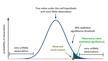
Here is a visual representation I’ve prepared. The example is with a commonly-used 95% threshold for the confidence level, equivalent to a one-sided p-value threshold of 0.05:

If the significance threshold for declaring an outcome statistically significant is for a p-value of 0.05 and the observed significance is a lower number, e.g. 0.04, then it can be said the result is statistically significant against the chosen null hypothesis.

Statistical significance is then a proxy measure of the likelihood of committing the error of deciding that the statistical null hypothesis should be rejected, when in fact, one should have refrained from rejecting it. This is also referred to as a type I error, or an error of the first kind. A higher level of statistical significance means there are more guarantees against committing such an error.

The more technically inclined might consider this deeper take on the definition and interpretation of p-values.

See this in action

Try itStatistical Significance Calculator
Robust p-value and confidence interval calculation.

Some might still be wondering: why would I want to know that, I just want to know if A is better than B, or vice versa?

What does it mean if a result is statistically significant?

A low p-value means a low probability of an outcome, or a more extreme one, to have occurred. Passing a low statistical significance threshold tells us that under the assumptions of the null hypothesis (e.g. the true effect is negative or zero) something very unlikely has occurred. Logically, observing a statistically significant outcome at a given level can mean that either one of these is true:

1.) There is a true improvement in the performance of our variant versus our control.
2.) There is no true improvement, but a rare outcome happened to be observed.
3.) The statistical model is invalid (does not reflect reality).

If are measuring the difference in proportions, as in the difference between two conversion rates, number #3 can be dismissed for all practical purposes. In this case the model is quite simple: classical binomial distribution, has few assumptions and is generally applicable to most situations. There remains a possibility that the distribution used is not suitable for analyzing a particular set of data. A common error I have witnessed is people trying to fit average revenue per user data into a calculation which allows only binomial inputs such as conversion rates.

Regarding #2: the lower the statistical significance level, the rarer the event. 0.05 is 1 in 20 whereas 0.01 is 1 in 100. Equivalently, the higher the statistical confidence level, the rarer the event. A 95% statistical confidence would only be observed “by chance” 1 out of 20 times, assuming there is no improvement.

What one hopes for that is #2 and #3 can be ruled out with the desired (low) level of uncertainty so #1 can remain the necessary conclusion. Knowing that a result is statistically significant with a p-value (measurement of statistical significance) of say 0.05, equivalent to 95% confidence, there still remains a probability of #2 being true. The good thing is that this probability is known given the A/B testing procedure and a worst-case scenario. This is how a p-value value and statistical significance serves as a measure of uncertainty.

If one is happy going forward with this much (or this little) uncertainty, then these are the quantifiable guarantees provided by testing.

It is probably as good a place as any to say that everything stated here about statistical significance and p-values is also valid for approaches relying on confidence intervals. Confidence intervals are based on exactly the same logic, except in the inverse. What is true for one, is true for the other. It is usually recommended to examine both the p-value and a confidence interval to get a better understanding of the uncertainty surrounding any A/B test results.

Significance in non-inferiority A/B tests

While many online controlled experiments are designed as superiority tests, that is: the error of greater concern is that a design, process, etc. that is not superior to the existing one will be implemented, there is a good proportion of cases where this is not the error of primary concern. Instead, the error that one is trying to avoid the most is that of failing to implement a non-inferior solution.

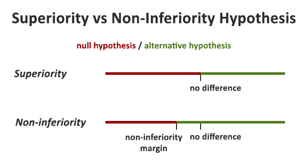
For example, when testing a simple color or text change on a Call-to-Action (CTA), the business won’t suffer any negatives if one color or text is replaced with another, as long as it is no worse than the current one, as in most cases it costs us nothing to have either. In other cases, the tested variant has lower maintenance/operational costs, so one would be happy to adopt it, as long as it is not performing significantly worse than the current solution. One might even be prepared to accept the possibility that it will perform slightly worse, due to the savings that would be made in the future. In cases like the above, a solution will be accepted as long as it can be proven not inferior to the existing one by more than an acceptable margin.

In these cases, the null hypothesis is defined as our intervention having a positive effect, or having a negative effect no larger than a given margin M: µ ≤ -M. The alternative hypothesis is that the changes proposed for implementation will have a positive effect or a negative effect smaller than M: µ > -M. M could be zero or positive. Naturally, in this case the interpretation of a statistically significant result will change: if a statistically significant result is observed the conclusion won’t be that there is true improvement of a given magnitude, but that the tested variant is just as good as our current solution, or better, and no worse than our chosen margin M.

To learn more on how to use such tests to better align questions and statistics in A/B testing, and to speed up your experiments, consult my comprehensive guide to non-inferiority AB tests.

Common misinterpretations of statistical significance

Falling prey to any of the below misinterpretations can lead to seriously bad decisions being made, so do your best to avoid them.

1. Treating low statistical significance as evidence (by itself) that there is no improvement

It is easy to illustrate why this is a grave error. Say only 2 (two) users in each group are measured in a given test. After doing the math the result is not statistically significant as it has a very high p-value of say 0.6 whereas a significance threshold of 0.01 was chosen.

Does this mean the data warrants accepting that there is lack of improvement? Of course not. Such an experiment doesn’t put this hypothesis through a severe test. The test had literally zero chance to result in a statistically significant outcome, even if there was a true difference of great magnitude. The same might be true with 200, 2,000 or even 200,000 users per arm, depending on the parameters of the test^[3:2.5].

In order to reliably measure the uncertainty attached to a claim of no improvement, the statistical power of the test should be examined. Statistical power measures the sensitivity of the test to a certain true effect, that is: how likely the test is to detect a real discrepancy of a certain magnitude at a desired statistical significance level. (“Power analysis addresses the ability to reject the null hypothesis when it is false” (sic) ^[2])

If the power is high enough, and the result is not statistically significant, reasoning similar to that of a statistically significant result can be used to say: “This test had 95% power to detect a 5% improvement at a 99% statistical significance threshold, if it truly existed, but it didn’t. This means there is good ground to infer that the improvement, if any, is less than 5%.”

2. Confusing high statistical significance with substantive or practically relevant improvement

This is erroneous, since a statistically significant result can be for an outcome so small in magnitude that it has no practical value. For example, a statistically significant improvement of 2% might not be worth implementing if the winner of the test will cost more to implement and maintain than what these 2% would produce in terms of revenue over the next several years. This can easily be the case for a small e-commerce business.

The above is just an example, as what magnitude is practically relevant is subjective and the decision should be made on a case-by-case basis. Here is what this would look like, with a accompanying confidence interval (read “Significance” as “Confidence”, the interval is from 0.4% to 3.6% lift):

The example is from our statistical significance calculator

This is considered by some to be a “failure” of statistical significance (it’s not a bug, it’s truly a feature!). The claim is that significance is a directional measure only, but that is wrong^[3:2.3]. A lower observed statistical significance (lower p-value, and hence higher confidence) in an A/B test is evidence of a bigger magnitude of the effect, everything else being equal. This demonstrates that a p-value is not just a directional measure but also says something about the magnitude of the true effect.

That said, it might be hard to gauge how big of an effect one can reasonably expect by statistical significance alone. It is a best practice to construct confidence intervals at one or several confidence levels to get a sense of the magnitude of the effect.

3. Treating statistical significance as the likelihood that the observed improvement is the actual improvement

Everything else being equal, observing a lower statistical significance (higher confidence) is better evidence for a bigger true improvement than observing a lower one, however, it would be a significant error to directly attach the statistical significance measure to the observed result. Having such a certainty would usually require much, much more users or sessions. Here is a quick illustration (read “Significance” as “Confidence”):

The example is from our statistical significance calculator.

While the observed lift is 20% and it has a high statistical significance, the 95% confidence interval shows that the true value for the lift is likely to be as low as 2.9% – blue numbers bellow % change are the confidence interval bounds.

To get a measure of how big and how small a difference can be expected, it is best to examine the confidence intervals around the observed value.

4. Treating statistical significance as the likelihood that the alternative hypothesis is true or false

This is a common misconception, which gets especially bad if mixed with misinterpretation #3. Forgetting that the alternative hypothesis is “A is better than control” and substituting it with “A is 20% better than control” (from the example above) on the fly makes for a perfectly bad interpretation.

Attaching probabilities to any hypothesis that tries to explain the numbers is not something that can be done using statistical significance or frequentist methods. Doing so would require an exhaustive list of hypotheses and prior probabilities, attached to them. This is the territory of Bayesian inference (inverse inference) and it is full of mines, so tread carefully, if you choose to explore it. My thoughts on the Bayesian “simplicity” temptation and other purported advantages of these approaches can be found in points #1 and #2 in “5 Reasons to go Bayesian in AB Testing: Debunked“, as well as “Bayesian Probability and Nonsensical Bayesian Statistics in A/B Testing”.

Common mistakes in using statistical significance in A/B testing

Any of these mistakes can invalidate a statistical significance test and the resulting error rates can easily be multiples, not percentages of the expected ones. Extra caution to avoid them is required. Using proper tools and procedures is one way to do so. For example, the user flow of the A/B testing hub has been designed to facilitate the avoidance of most such missteps.

What is common in these mistakes is that the nominal (reported) statistic, no matter the type and label: significance, confidence, p-value, z-value, t-value, or confidence interval, does not reflect the true uncertainty associated with the observed outcome. The uncertainty measure becomes useless or introduces significant and hard to measure bias. As the saying goes: Garbage In, Garbage Out.

1. Lack of fixed sample size or unaccounted peeking

This mistake happens when:

• using a simple significance test to evaluate data on a daily/weekly/etc. basis, stopping once a nominally statistically significant result is observed. While it looks OK on the surface, it is a grave error. Simple statistical significance calculations require fixing the sample size in advance and only observing the data once at the predetermined time or number of users. Do differently, and the uncertainty measure can be thrown off by the multiples. As this issue may not be immediately obvious, consider a detailed discussion at “The bane of A/B testing: Reaching Statistical Significance“.
• the sample size has been decided in advance, but peeking with the intent to stop happens regardless
• using a proper sequential testing method, but failing to register your observations faithfully, so that the statistics can be adjusted accordingly
• using a Bayesian sequential testing method that claims immunity to optional stopping (why Bayesian approaches are not immune to optional stopping)

How to avoid peeking / optional stopping issues?

One way is to fix the sample size in advance and stick to just a single observation at the end of a test. It might be inflexible and inefficient, but the result will be trustworthy in that it will show what is warranted by the data at hand. Alternatively, a sequential testing methodology can be used such as the AGILE A/B testing approach. Our A/B testing calculator is available to make it easy to apply it in daily CRO work. With sequential evaluation one gains flexibility in when to act on the data which comes with added efficiency due to the 20-80% faster tests.

2. Lack of adjustments for multiple testing

Multiple testing, also called multivariate testing or A/B/n testing, is when more than one variant is tested against a control in a given test. This can lead to increased efficiency in some situations and is a fairly common practice, despite the drawback that it requires more time/users to run a test. Analyzing such a test by either picking the best variant and doing a t-test / z-test / chi-square test, etc. on the control and that variant, or doing one such test for each variant against the control significantly increases the Family-Wise Error Rate (FWER). The more hypotheses being tested, the greater the chance of getting a false positive.

There are special procedures for accounting for this increase and reporting p-values and confidence levels which reflect the true uncertainty associated with a decision. Dunnett’s post-hoc adjustment is the preferred method. It is also the one used in AGILE A/B testing. For more, read our detailed guide to multivariate testing which covers when such a test is more efficient, among other things.

3. Lack of adjustments for multiple comparisons

Multiple comparisons happen when there is more than one endpoint for a test. It is another example of increasing the Family-Wise Error Rate. For example, in a single test the statistical significance on all of the following measures is computed: bounce rate differences, add to cart conversion rate differences, purchase completion conversion rate differences. If one is statistically significant, the variant is implemented.

This is an issue since doing more than one comparison between the groups makes it more likely that one of them will turn out statistically significant than the p-value and confidence or significance level reported. There are different procedures for handling such a scenario. The classic Bonferroni correction should be the preferred one. Benjamini-Hofberg-Yekutieli’s false discovery rate procedures can also be considered, but I believe them to be generally inappropriate for the typical A/B testing scenario.

Bonus mistake: using two-tailed tests and interpreting them as one-tailed tests. This is very common, especially since a lot of vendors seem to be using and reporting two-sided significance. I’ve written a whole separate article on this here: one-tailed vs. two-tailed significance tests in A/B testing.

How to choose an appropriate statistical significance level?

Many people have trouble when it comes time to choose the statistical significance level for a given test. This is due to the trade-offs involved. The major trade-off is between speed, flexibility, and efficiency on one side, and accuracy, certainty, sensitivity and predictability on another.

The major trade-off in A/B testing is between speed, flexibility, and efficiency on one side, and accuracy, certainty, sensitivity, and predictability on another.

No matter what kind of statistical method is being used, the following trade-offs are inevitable:

• increasing the required statistical significance threshold means increasing the required sample size, thus slower testing;
• increasing the certainty about the true difference, equivalent to decreasing the width of the confidence interval, means increasing the required sample size, thus slower testing;
• increasing the statistical power (test sensitivity to true effects) means increasing the required sample size, thus slower testing;
• decreasing the minimum detectable effect size means (with a given power and significance) means increasing the required sample size, thus slower testing;
• increasing the sample size (time to run a test) means better certainty and/or higher test sensitivity and/or the same sensitivity towards a smaller effect size.

Significant detail about the different trade-offs in AGILE A/B testing, many of which apply to any kind of A/B test, is available in “Efficient AB Testing with the AGILE statistical method” (go straight to the “Practical guide” part, if you prefer).

See this in action

Try itA/B Testing Calculator
Advanced significance & confidence interval calculator.

Several questions emerge quickly even from the brief summary above. Questions like: Shall I test longer, for better certainty, or should I test faster, accepting more frequent failures? Should I run quick, under-powered tests, seeking improvements of significant magnitude while missing smaller opportunities? Unfortunately, there are no easy answers in A/B testing methodology about what values to choose for the main parameters of a statistical test.

Contrary to popular belief, the answers don’t get easier if there are more users and sessions at one’s disposal (huge, high-trafficked site), nor do they become especially harder with small sites that barely get any traffic and conversions.

That is because while high-trafficked and high-converting sites have more users to run tests on, it usually also means that even the slightest improvements can result in many thousands or even millions of dollars worth of revenue or profits. This warrants running highly sensitive tests, and high power quickly ramps up the user requirements to levels where even the most visited sites on earth need weeks or months to run a proper test. Making even small errors is equally costly, pushing statistical significance requirements higher, and thus slowing down testing even further.

Conversely, having few visits and conversions means that one must aim for big improvements in whatever is being attempted, if A/B testing is even going to be worth it. On the other hand, if a business is small AND nimble, it can accept higher uncertainty in any action, or be able to test so fast, that the lower sensitivity is not such a great issue.

My advice is to weigh the costs for designing, preparing and running the A/B test against the potential benefits (with a reasonable future extrapolation, e.g. several years) and see the sample sizes (and thus time) required by several different combinations of values for the three main parameters (significance, power, minimum effect size). Then, choose a statistical design that hits closest to the perfect balance. Using a flexible sequential testing framework such as AGILE can make the decision on the minimum effect size much easier, since in case the true difference is much larger or much smaller, the test will simply stop early so the efficiency sacrificed will be minimal.

There are some good practices that should be followed irrespective of what the sample sizes allow. For example, analyzing (sequential) tests on a weekly basis and not running tests for less than a week. For many businesses Tuesdays are not the same as Sundays, and even if a satisfactory test can be run in 3 days, better plan it for a full seven days. Other best-practice advice can be found in white papers and books written by experts in the field.

While there is no recipe for a perfect A/B test, the above advice for making a choice while facing several trade-offs should be a helpful starting point for CRO and UX practitioners.

See this in action

Try itA/B Testing Hub
The all-in-one A/B testing statistics solution

(Added Apr 27, 2018): I have subsequently developed a comprehensive overview of the costs & benefits and risks & rewards in A/B testing and have built a tool that will do the balancing act for you, allowing you to use A/B testing to manage business risk while maximizing gains and rewards: the A/B Testing ROI Calculator.

(Update Feb 2022): Since December last year this tool has become an integral part of planning ROI-optimal tests using the A/B testing hub.

Closing thoughts

While statistical significance testing is a powerful tool in the arms of a good CRO or UX expert, it is not a panacea or substitute for expertise, for well-researched and well-designed tests. It is a fairly complex concept to grasp, apply appropriately, and communicate to uninformed clients. I hope this post, which is a natural continuation of years of work on A/B testing statistical theory and methodology, helped shed light on it and can serve as a handy introduction to the matter.

References:

1 Aberson, C. L. (2010) – “Applied Power Analysis for the Behavioral Sciences”, New York, NY, Routledge Taylor & Francis Group
2 Fisher, R.A. (1935) – “The Design of Experiments”, Edinburgh: Oliver & Boyd
3 Mayo, D.G., Spanos, A. (2010) – “Error Statistics”, in P. S. Bandyopadhyay & M. R. Forster (Eds.), Philosophy of Statistics, (7, 152–198). Handbook of the Philosophy of Science. The Netherlands: Elsevier.

About the author