A/B Testing Statistics – A Concise Guide for Non-Statisticians

Navigating the maze of A/B testing statistics can be challenging. This is especially true for those new to statistics and probability. One reason is the obscure terminology popping up in every other sentence. Another is that the writings can be vague, conflicting, incomplete, or simply wrong, depending on the source. Articles sprinkled with advanced math, calculus equations, and poorly-labeled graphs represent a major hurdle for newcomers.

I faced these very problems in early 2012. Now, with years of experience as a developer of statistical software at Analytics-Toolkit.com, a lecturer and consultant in A/B testing statistics, and after writing the book “Statistical Methods in Online A/B Testing”, I think I’m in good position to produce an accessible introduction to statistics in A/B testing. Hopefully without the aforementioned issues!

If you are just getting started in the field or if your job involves CRO and online experimentation in a cursory way, this concise guide should be a good introduction to the discipline. The article covers the following:

1. Why A/B test?
2. The role of statistics in A/B testing
3. Key A/B test statistics
4. Confidence intervals
5. Introduction to statistical hypothesis testing
6. Types of errors in null hypothesis testing
7. P-values and statistical significance
8. The effect of statistical power on test statistics
9. Bayesian probability and “chance to be best”
10. How to interpret A/B test statistics
11. Caveats in applying statistical methods
12. How to ensure the reliability of test statistics
13. Further reading and resources

All of the topics discussed are supported by inline references which can be a good starting point for a deeper dive.

Why A/B test?

A/B testing is the process of randomly assigning users to a control group and one or more treatment groups, and measuring the difference between the outcomes in the control group and the treatments. A “treatment” is any change or intervention that can be introduced.

Its more scientific name is a “randomized controlled experiment”. An experiment differs from simply making changes and observing associated shifts and drifts in relevant time series. Its main benefit is that an experiment allows for a causal link to be established between the change and any observed effect (or lack thereof).

The above is not possible without an A/B test. The reason is that there is no other reliable way of measuring and accounting for the variability in a time series caused by other known or unknown factors.

The main goal of A/B testing, regardless if it is applied as part of a CRO or UX process, is as a tool for managing the business risk associated with change and innovation. Part of achieving that goal is to estimate with some precision the effect of a proposed change which is where statistics take the spot.

An example of a change that can be A/B tested is the addition of a payment method to an e-commerce store. The effect may be an increase or decrease in the average revenue per user. This example will be referred to in the rest of the article.

The role of statistics in A/B testing

To achieve their goal, A/B tests must account for the variability of outcomes. This observed variability is due to differences between people and in people’s behavior over time. Given the limited time and number of people that can be included in an experiment, as well as measurement errors, observed variability is characteristic of all processes involving human behavior. As a result, the observed decrease or increase in the metric of interest may differ from the actual state of the world in a non-trivial way.

Statistical estimates (a.k.a. “statistics”) produce statements about the true effect of a change or provide a measure of uncertainty associated with such statements. The uncertainty being caused by the abovementioned variability.

One the most basic and widely used statistics is the observed difference between a variant and a control in a test. It is typically expressed as a relative percentage change, also known as “lift”. For example, if the average revenue per user in the control is observed to be $10 and the average revenue per user in a treatment group is $12, then the relative percent change is $12/$10 = 0.20 = 20%. Equivalently, it can be said that “the lift is 20%”, but it gets awkward to use “lift” if the observed change is negative, e.g. “-5% lift”.

While the observed values for average revenue per user are $10 and $12, the actual values might be $11 and $10.5 respectively, the difference being due to the variability inherent to the testing process.

The above is an example of a non-trivial difference since it can completely reverse our interpretation of the test. However, there is nothing in the observed outcome which hints at this probability. That is why additional statistics need to be reported for each A/B test.

Key A/B test statistics

Important A/B testing statistics used to convey information about the uncertainty associated with an observed outcome include:

• p-values
• confidence levels
• confidence intervals

Such statistics are used in A/B testing to estimate and communicate the level of uncertainty introduced by the variability of outcomes which is caused by the inherently variable human behavior, as well as measurement error.

A common feature of these statistics is that they measure and express variability inherent to the data generating process. “Data generating process” is a catch-all term encompassing everything relevant to how the data is produced, captured, processed, and analyzed. This is important for the correct interpretation of the various statistics, as well as their assumptions and caveats.

A comprehensive yet accessible explanation of these statistics can be found in p-values and confidence intervals explained. Below is an abridged version covering all important points from a practical standpoint.

Confidence intervals

Confidence intervals express the range of uncertainty surrounding an estimate produced by a specific test at some specified confidence level. For example, the observed lift (relative percentage change) may be 20%, with a 95% interval bound at -3%, as shown below.

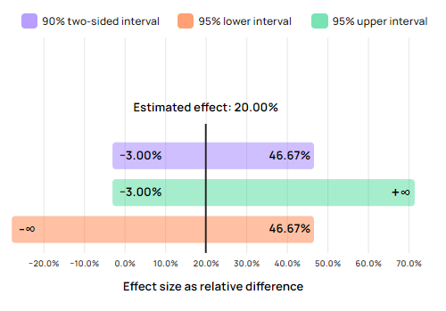
This means that if the true effect was indeed exactly 20%, given the A/B test data at hand it would not have been surprising to see an outcome as low as -2% or 0% or +3%. The “data at hand” term includes, most importantly, the number of users observed in both the control group and the group experiencing the treatment. The more users, the less uncertainty associated with any observed outcome.

Assume, for example, that the above 3% bound was obtained with 10,000 users per group. Had the test included 50,000 users per group instead, the bound would have been at 6% with the same observed outcome of 20% lift:

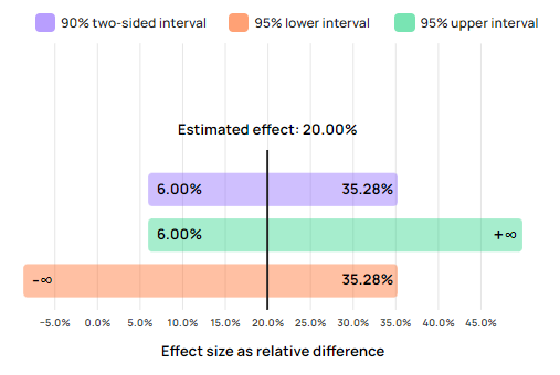
The range from +6% to plus infinity includes fewer values than the range from -3% to plus infinity. Equivalently for the 90% confidence interval which spans -3% to 46.67% in the first case, compared to just 6% to 35.28% in the second. This is due to the increased number of users included, known in statistics as the “sample size”.

Such visual representation of the uncertainty surrounding the estimate can help facilitate decision-making, as examined below.

The confidence level of an interval signifies the probability of the testing procedure to result in an interval which covers (includes within its bounds) the true value. For example, a 99% confidence interval would contain the true difference in average revenue per user in 99% of hypothetical test outcomes. While 90%, 95%, and 99% confidence intervals are typically reported in statistics software, one can also compute and plot a confidence interval at any confidence level between 0% and 100%.

How to use confidence intervals?

Put simply, values outside a confidence interval of an adequate confidence level are considered rejected by the testing procedure at that level. Values inside the interval remain within the region of uncertainty and cannot be ruled out.

Continuing the example, the 95% interval bound at -3% means one cannot reject values above -3% such as 0% with the available data. The statistical test does not offer convincing evidence for such a rejection. In the second example where the 95% interval bound is at 6%, the data offers sufficient evidence to reject any value below 6%, including 0%.

Introduction to statistical hypothesis testing

The other main A/B testing statistics: p-values, confidence levels, and the concept of statistical significance require a short dive in hypothesis testing. While one goal of A/B testing is to pinpoint the true effect of a change, a more modest and practical goal might be to simply establish lack of negative effect or lack of no effect. Oftentimes pursuing such a goal results in better return on investment from testing, compared to getting a highly accurate lift estimate.

Hypothesis testing is a great tool for accomplishing the above goal, and statistical hypothesis testing (a.k.a. Null Hypothesis Statistical Testing or NHST) is needed in A/B testing due to the inherent variability of outcomes.

Hypothesis testing starts with the definition of a loose substantive claim which is then framed as a more precise substantive hypothesis in terms of a given metric, which is then translated into a statistical hypothesis with specific model assumptions.

A substantive hypothesis is therefore just a claim about the effect of a given change framed in terms of a suitable metric. In our example A/B test the substantive hypothesis is that “the addition of a new payment method X by a particular implementation Y will result in some increase in average revenue per user”. This hypothesis is called the “alternative hypothesis”. As in “alternative to the status quo”.

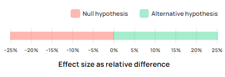
Someone arguing against this hypothesis would claim that the addition of the new payment method in said way would in fact harm revenue, or it might have no effect whatsoever. This type of claim is in favor of business as usual and is referred to as the “null hypothesis”.

Different reasons could be put forth in support of such a default claim. Users might simply not care or the implementation might be such that users remain oblivious to the new option due to poor user design. Adding a new payment method might result in overwhelming the user due to the many choices presented.

However, a claim critical towards a proposed positive effect might not cite any reason whatsoever since by default the burden of proof is on whoever proposes a change that might disrupt existing revenue streams.

Due to a philosophical issue known as “The Problem of Induction” one cannot directly prove their claim regardless of how much data is available. However, one can refute an opponents’ claim through a statistical hypothesis test if its outcome contradicts said claim. Typically the null hypothesis is considered “a safe bet” and rejecting it on probabilistic grounds is the main goal of statistical hypothesis testing.

It is here that A/B testing statistics play a critical role. The null hypothesis will be rejected by a given test if its outcome is statistically significant. To determine if a test outcome is statistically significant however requires first setting a statistical significance threshold. This threshold controls the false positive error rate from the point of a worst-case scenario in which the null hypothesis is in fact true.

A textbook value is to have a 0.05 p-value threshold, or, equivalently, a 95% confidence level threshold, but ideally a choice would be made to set this threshold while planning the test and considering the trade-off between the two possible types of errors.

Types of errors in null hypothesis testing

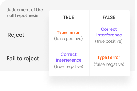
Two types of errors are possible as a result of performing a statistical hypothesis test. One is to falsely reject a true null hypothesis, and the other is to fail to reject a false null hypothesis. Common terms for these are “Type I” and “Type II” errors, as well as “false positive” and “false negative”.

Estimating and controlling these error probabilities is the main goal of statistics such as p-values, observed confidence levels, and confidence intervals.

Determining a test plan includes balancing the probability of a false positive with that of a false negative. Decreasing the probability of one error increases the probability of another, everything else being equal. The only way to reduce both is to increase the test’s sample size, or in this case the number of users assigned to each test variant. However, this comes with increased business risks and is subject to decreasing marginal return from testing.

Determining the correct test duration and sample size, as well as the statistical significance threshold should ideally be done by a trained analyst with the help of specialized software such that an optimal balance between business risks and rewards is achieved. This is outside the scope of the current article, but you can read more in the glossary entry on risk-reward analysis and the references therein.

P-values and statistical significance

A p-value is a test statistic which estimates a worst-case probability for committing a type I error. As described above, a type I error is falsely rejecting a true null hypothesis, or a false positive. Incorporating an estimate of the uncertainty of the test procedure, it produces a probability of observing an outcome as extreme or more extreme than the observed.

Simply put, a p-value expresses how surprising it would be to observe an effect as large or larger than the observed, assuming the null hypothesis was in fact true. The more surprising an outcome, the greater the weight of evidence against the null hypothesis provided by the A/B test. A lower p-value means a more surprising outcome and a more preposterous coincidence in observing it had there been no effect or a negative effect (in our example).

Being a probability, a p-value can span from 0 to 1. A value very close to zero means a very low probability, while a value close to one represents a very high probability.

Continuing the e-commerce store example, an A/B test with 10,000 users with an observed outcome of 20% lift would have reported a p-value of 0.0762:

0.0762 is not a high p-value. As an A/B testing statistic it shows the probability of committing a type I error by taking is non-trivial. If the statistical significance threshold was set to 0.05 then a p-value of 0.0762 would not pass it. The outcome would not be statistically significant, hence the null hypothesis would not be rejected.

In the A/B test with 50,000 users per test group the same 20% lift results in a p-value of 0.0094. This reflects an extremely low probability of seeing such a lift if the true effect was zero or negative. In most scenarios such a value would be interpreted as statistically significant and the null hypothesis would be rejected in favor of the alternative.

The confidence level statistic

In online A/B testing it has become a convention due to early adopters to report a confidence level equivalent to the p-value instead of or in addition to the p-value itself. The respective confidence level is shown in each of the above two screenshots in the “Confidence” column.

As a statistic, “Confidence” is the confidence level of a confidence interval such that it barely excludes the null hypothesis. Mathematically it a simple transformation of the p-value:

% confidence = (1 – p) * 100

It is easy to see how in the first example the confidence percentage is (1 – 0.00762) * 100 = 0.923790 * 100 = 92.3790%. If the confidence threshold was 95% then 92.3790% < 95% so the outcome is once again not statistically significant.

How to use p-values and confidence?

A p-value or its corresponding confidence level can be compared to the predetermined statistical significance or confidence threshold. If a p-value statistic is below the significance threshold, the null hypothesis is to be rejected in favor of the alternative. Likewise if the confidence level is greater than the confidence threshold.

If a result is not statistically significant, the default situation is to remain in place since the A/B test did not provide sufficient evidence to reject the null hypothesis. Given the null in our example is that of zero or negative true effect, it is equivalent to state that the experiment did not provide sufficient evidence against the possibility of a negative impact from the tested change.

Notably, the reverse logic does not apply. A statistically non-significant outcome due to a high p-value is not to be used as evidence that there is no effect or that there is a negative effect. Without going into details, a test might provide such evidence only to the extent to which the procedure was able to rule out certain non-zero effects which is reflected in the statistical power towards various discrepancies from zero.

See this in action

Try itA/B Testing Hub
The all-in-one A/B testing statistics solution

The effect of statistical power on test statistics

A brief note on statistical power is warranted, even though it is not really an A/B testing statistic, but rather a characteristic of a statistical hypothesis test.

Statistical power is the sensitivity of a statistical test against particular true effect sizes. The more sensitive a test, the smaller true effects it can detect as statistically significant. All else being equal, a test is more sensitive if it has a larger sample size.

In A/B testing, greater power means less uncertainty of all statistical estimates. More powerful tests result in narrower confidence intervals. They produce smaller p-values if the true effect is not contained in the null hypothesis parameter space.

Power calculations against various possible or probable true effect sizes are useful when planning an A/B test in terms of sample size and duration, and play a key role in balancing the risk versus reward for the business. Power analyses after a test has started can be useful in a limited number of very specific situations. So-called “post-hoc power” is a meaningless concept and should not be employed. This is covered in much more detail in my book.

Bayesian probability and “chance to be best”

Proponents of Bayesian approaches to A/B testing have been very vocal in propagating a number of false claims of benefits of Bayesian statistics as well as supposed drawbacks of frequentist statistics. Hence they’ve earned a spot in this overview of A/B testing statistics. Feel free to skip this section if not of interest.

Briefly, Bayesian statistics revolve around calculating inverse probabilities in which one mixes subjective opinions with the data to produce subjective probabilities as outcome. These supposedly reflect the way the data from an A/B test should cause one to change their views. In other views, Bayesian statistics produce odds that a given change will outperform the current implementation. Supposedly the benefit is that you perform tests in a way which balances business risk and reward. The major characteristic is the mixing of decision-making and statistical estimation and statistical inference.

Bayesian statistics include posterior probability distributions, posterior odds, Bayes factors, and credible intervals. These are often masked by terms such as “probability to outperform”, “probability to be best”, “chance to beat original”, and so on.

Frequentist statistics, represented by statistics such as p-values, confidence levels, and confidence intervals, provide objective probabilities. Frequentist statistics are as free from subjectivity as possible and can be plugged into any decision-making view or framework. Prior knowledge or opinions can influence the design of the test, but are never incorporated in the resulting statistics which aim to reflect the evidence of the data. No more and no less. Decision-making to achieve optimal returns and statistical estimation and inference are separate tasks, as they should be.

While theoretically there can be value in using Bayesian estimates, it is incredibly difficult to employ them in practice, even for personal decision-making. Let alone when one requires statistics which would be accepted by a wider group.

This is perhaps why I’m not aware of a prominent A/B testing tool on the market which actually implements Bayesian inference and estimation. Many now claim to do so, but that task is impossible unless one can specify their prior probability distribution and I am yet to find a tool that does that. I think it is not a coincidence that the major feature of a Bayesian approach is absent in these tools.

Further exacerbating the issue, many tools employing these quasi-Bayesian statistics commit the error of assuming Bayesian methods are immune to peeking, which is untrue.

In my view the so-called Bayesian statistics reported by most tools do not live up to their name (certainly not their labels), are deeply flawed, and cannot be usefully interpreted. This is why I find it pointless to try and explain how they can be used in a fruitful manner.

For in-depth reasons why Bayesian estimates are not covered in more detail here, see the following articles: Frequentist vs Bayesian Inference, Bayesian Probability and Nonsensical Bayesian Statistics in A/B Testing, 5 Reasons to Go Bayesian in AB Testing – Debunked. For a selection of questionable and outright false claims regarding Bayesian and frequentist statistics read The Google Optimize Statistical Engine and Approach.

How to interpret A/B test statistics

Here is a brief recap on interpreting the key statistics used in A/B testing.

• Use confidence intervals to judge how much uncertainty there is surrounding any observed test outcome. Values outside the interval can be excluded with a confidence level equal to that of the interval, e.g. 95%.
• Use p-values to reject claims that if true would hinder the adoption of the proposed change. The lower the p-value, the lower the probability of falsely rejecting such claims.
• Confidence, or the observed confidence level is a mirror of the p-value. Higher confidence means there is less uncertainty in the evidence in favor of rejecting the null hypothesis.
• If a p-value is higher than the desired significance threshold, or a confidence level is lower than a desired confidence threshold, do not implement the tested variant.

Caveats in applying statistical methods

There are multiple caveats in calculating and applying the different statistics in A/B testing. Most of them refer to the correspondence of the statistical model to the problem at hand. This happens since all statistics calculations come with embedded assumptions regarding the data generating process.

Here are a few of the most important ones to watch out for:

• Measure the right metric. Conversion rates make for good metrics, consider averages such as average revenue per user (ARPU). User-based metrics should be preferred to session-based ones.
• P-values and confidence intervals should correspond to the tested claims. A typical error is using two-sided p-values and intervals instead of one-sided ones. The former apply to most practical situations.
• If interested in making claims regarding relative difference (% lift), make sure to compute p-values and confidence intervals for relative difference and not absolute difference.
• Comparing multiple variants versus a control in a test (A/B/N test) requires additional adjustments to arrive at accurate statistics.
• Simple statistics work for simple scenarios only. Evaluating the data as it gathers is a complex task involving special stopping bounds and sophisticated adjustments to all A/B testing statistics, including p-values, confidence intervals, and point estimates. Otherwise, peeking occurs and statistical guarantees are out.

Violating key model assumptions behind the methods can render the reported statistics worse than useless, due to the false sense of certainty they can provide. To avoid reporting inaccurate statistics plan tests carefully with understanding of the methods being used and the prerequisites for their application.

How to ensure the reliability of test statistics

Regardless if one uses in-house tools or third-party tools, there are a few common tips to ensure the reliability of A/B testing statistics used in decision-making.

First, there should be transparency about the methods used as well as key assumptions behind them. This should ensure accurate communication of the uncertainty in the data and facilitate actual risk management.

Second, the tools should be able to demonstrate their error guarantees. A great way to assess their performance is through a series of A/A tests, ideally several hundred or several thousand. Examining the outcomes will also be a great exercise in deepening the understanding of statistical hypothesis testing and estimation through experimentation.

And finally, the tools should have in-built mechanisms for checking the reliability of each individual test. A sample ratio mismatch check is a must-have for any tool. Automatic checks of any other assumptions should be employed where possible.

Further reading and resources

The above is a gentle introduction to the design of experiments and statistical testing and estimation. A/B testing and experimentation in general is often considered one of the most difficult disciplines to break into and master, so if your interest in the matter is serious, consider some of the resources highlighted below.

Free online reading resources:

The glossary of A/B testing terms at Analytics Toolkit contains short and accurate definitions of over 220 terms used in A/B testing, especially related to the statistical analysis of experimental data.

Over 70 in-depth articles on varying A/B testing topics can be found in this blog. Also consider our white papers on A/B testing statistics.

Microsoft’s Exp Platform organizes articles, publications, and a few videos where experimentation professionals from the Microsoft team share their learnings from the many tests ran there. Mostly deep and good stuff, though some of it is not really applicable if you are a smaller business or just getting started with A/B testing.

Books:

A deep exploration of A/B testing statistics and risk-management through experimentation is offered in my book “Statistical Methods in Online A/B Testing”. It is meant as an accessible and fairly comprehensive methodological reference for A/B testing practitioners and aspiring data scientists.

“Trustworthy Online Controlled Experiments” offers a detailed presentation of best practices for running an experimentation program, with examples from Microsoft’s experimentation practices as well as other online giants such as Google, Amazon, and others.

“Statistical Inference as Severe Testing” contains an accessible and extremely insightful philosophical examination of experimentation and testing methodology. Its discourse focuses on scientific experiments, but everything in the book applies equally well to business experiments, including online A/B testing.

Tools:

Analytics-Toolkit.com offers a free trial which you can use to explore different concepts in practice and also tap into the vast knowledge and experience which went into building it. The detailed contextual help in the A/B testing hub and the different statistical calculators, as well as the Knowledge Center can both serve as resources.

GIGAcalculator offers a number of free statistical calculators covering all test statistics discussed above, and more. Functionalities may be somewhat limited and confined to simpler scenarios, but it should be a great starting resource.

About the author