
Hundreds if not thousands of books have been written about both p-values and confidence intervals (CIs) – two of the most widely used statistics in online controlled experiments. Yet, these concepts remain elusive to many otherwise well-trained researchers, including A/B testing practitioners. Misconceptions and misinterpretations abound despite great efforts from statistics educators and experimentation evangelists.
I should know. I’ve written a book, produced a course, and hundreds of articles on this very topic. Statistics-related questions arrive in the support inbox of Analytics Toolkit on a daily basis and some exhibit similar issues.
What seems missing is a reasonably short, understandable, yet accurate account of p-values, confidence intervals, and their utility. That is no coincidence. Coming up with such a piece is a massive challenge. Below is my attempt to take it on with an article aiming to be accessible to anyone with a basic background in A/B testing.
Variability and randomized experiments
Imagine a typical online controlled experiment where users are randomly assigned to two test groups. One is the control group, and the other is the variant which implements a proposed change.
The main parameter of interest is a relative difference between the variant and the control group, typically expressed as percentage lift. The metric of interest is the purchase rate per user. The goal of the test is to estimate the effect this change has on users. To aid decision-making, the possibility that the change is going to have no effect or a detrimental effect on the business has to be ruled out within reason.
The problem is the presence of variability in the behavior of users both across time, and from one user to another. No two people are the same, and even the same person might react differently depending on when they are experiencing the tested change.
As a result, measuring the effect of a change of a fraction of users will produce an outcome that will likely differ from the actual effect on all users that comprise the target population. This is what is known as variability in outcome. The variability in outcome is only exacerbated by any measurement errors that might occur such as lost data, inaccurate attribution, loss of attribution, and so on.
As a consequence, no matter how many users are measured, a possibility remains for the observed effect to differ from the actual effect.
One possible way of dealing with variably is to try and eliminate or reduce it. One can attempt to balance the number of users with a certain characteristic that end up in one test group or the other. However, the possible reasons behind the variability are practically infinite, making it impossible to know or attain balance on all relevant characteristics.
Another approach is to simply account for variability in the process of data evaluation and interpretation.
Two things make this second approach feasible. First, though infinitely many, the combined effect of all sources of variability is not infinite itself. The total variability is bounded by the actual effect size. And second, randomizing users across the test groups means that what group they end up in is independent of their propensity to purchase.
These characteristics of randomized controlled experiments enable the computation of reliable statistical estimates.
The random assignment of users in test groups enables the calculation of objective error probabilities despite the potentially countless sources of variability.
Randomization makes the multifactor variability in outcome easy to model, estimate, and present in the form of p-values and confidence intervals.
What is a point estimate?
Understanding point estimates is crucial for comprehending p-values and confidence intervals. A point estimate in the setup described above is equivalent to the observed effect. Therefore, the observed effect is the point estimate of the true effect. For example, the observed test outcome might be +10% and that is also the point estimate. The true effect is typically unknown, except in simulations.
The observed effect is a random variable and due to the randomization procedure its variability is easy to estimate. An example of the variability of the observed effect is demonstrated below by hypothetical repetitions of the same exact experiment with a true value of the difference between the variant and control of exactly 10% (click on all images to view in full size).
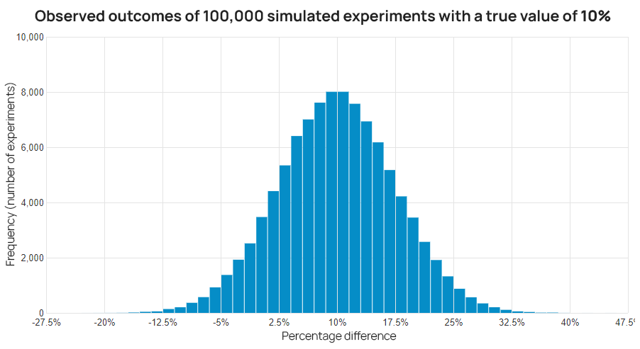
The above shows why the observed effect should never be mistaken for the actual effect. Whatever result is observed in the A/B test is just a best guess as to what the true effect of the change is, given the number of users in the test.
It is “best” in a non-trivial sense. In the face of variability a point estimate:
- reflects all information about the true value that there is in any particular sample is reflected
- has the highest possible probability of being close to the true effect size
- is not systematically biased against any possible true effect size
- would have most likely been closer to the true effect size, had we observed more data
Not all of the above characteristics may be present for point estimates in all types of tests. However, the last one should always apply and has important implications. Notably, the same observed outcome coming from two A/B tests, one with fewer users than the other, would warrant a different interpretation. A point estimate would be more or less reliable, depending on how many users it was based on.
A point estimate is the best guess of the true effect size given the variability at play. Its observed value is subject to random variability which is less pronounced with a greater number of users in a test.
What is a confidence interval?
A confidence interval (CI) expresses the variability associated with the claim that the observed effect is the actual effect, given certain data. It is calculated by computing all possible ways the particular A/B test might have turned out, assuming the true effect was equal to the observed one.
The result of the calculation can be plotted as a distribution of outcomes with different probability of occurring, the same way it is done for a point estimate.
A desired proportion of said distribution can then be cut out as being less probable than a given threshold. For instance, one can cut out all values with probability of occurring of less than 1%. What remains above the cutoff is a 99% confidence interval. A 99% confidence interval is an interval with a confidence level of 99%.
A confidence interval visualizes the variability of a point estimate at a certain level by producing one or two bounds expressed in terms of possible effect sizes.
This cut will occur at different values depending on how large the variability of the estimate is. A larger sample size means lower levels of random variability.
For example, with an observed effect of +10% lift a 95% interval cutoff might be at -3.5% if it came from a test on 12,000 users.

The same 10% resulting from a test on 50,000 users would have a 95% interval bound at +3.25% since the variability of the estimate is smaller due to the larger sample size.
Since intervals are dependent on the point estimate with its random variability, intervals themselves exhibit random variability.
The utility of using a confidence interval for the effect size is that it expresses a particular level of variability as a range as opposed to just a point. Outcome values covered by the interval would not be considered as surprising if the true effect size is indeed equal to the observed, whereas values outside the interval would be. The fewer values covered by the interval, the less variability it represents.
Using the numbers above, with 10,000 users one would have a hard time ruling out the possibility that the true effect is negative, despite the observed change of +10%. However, with 50,000 users and the same result of +10%, the uncertainty in claiming lack of a negative effect is much smaller, as demonstrated by the 95% bound at +3.25%.
Does it mean there remains no chance of the true effect being negative? Of course not. For example, the 99.5% bound with 50,000 users is at -0.57%, meaning that at the 99.5% confidence level an outcome of 0% would not have been surprising.
What is a p-value?
A p-value can be viewed as examining the observed effect and its variability through the lens of the supporter of a certain claim.
In this A/B test a major claim of interest is “the change has no effect or a detrimental effect on the business”. In terms of percentage lift this claim corresponds to a lift of zero percent or less. The claim can be rejected if the experiment’s data disagrees with it to a significant extent.
To calculate the p-value relating the above claim and the observed effect size:
- calculate all possible outcomes of the A/B test at hand, assuming the lift is exactly zero percent
- determine how many of these result in a value as large as the observed, or larger*
- divide the result of (2) by that of (1)
The resulting proportion represents an objective estimate of the rarity of the observed outcome, or more extreme ones, assuming the claim was true. In the graph below, it is visualized as the proportion of the blue area right of the actual observed outcome from the total blue area.
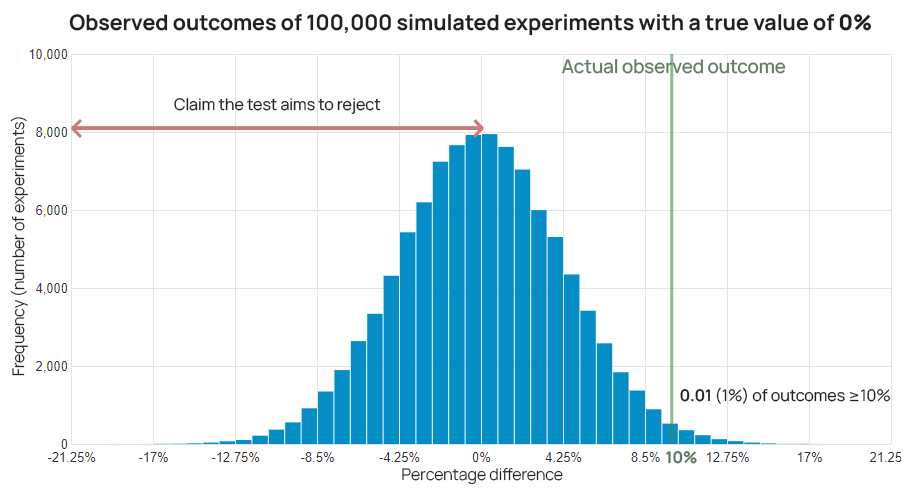
For example, if an outcome of 10% lift results in a p-value of 0.01 means that outcomes greater than or equal to 10% would be observed in only 1 out of every 100 possible test outcomes, were the lift actually zero or negative. In other words, seeing a 10% lift would be quite unexpected with a true effect of zero or less.
The more unexpected the outcome, the harder it is to argue for the tested claim. In this way a p-value is useful as part of a procedure for rejecting a claim in the face of variability with certain error guarantees.
A p-value reflects the evidence the outcome of a test provides against a given claim, while accounting for the variability associated with the test procedure.
A low p-value means the test procedure had little probability of producing an outcome equal to or greater than the observed, were the claim it was constructed under true. Yet it produced such an outcome. The surprising outcome begs for an explanation from anyone supporting that claim and may serve as ground to reconsider if the effect is negative or zero.
Another way to look at a p-value is that it shows how often one would be wrong in rejecting a particular claim with the given test outcome and associated variability, were that claim true.
* the probability of observing any exact value is always infinitely small, which is why one is instead interested in the combined probability of observing any outcome as large as the observed, or larger
See this in action
The all-in-one A/B testing statistics solution
Closing remarks
This was my attempt at explaining p-values and confidence intervals, two of the most important A/B testing statistics, in an accessible and useful manner, while staying true to the core concepts. It deliberately features a basic scenario, making it possible to skip the dozens of asterisks that would have been needed otherwise. It purposefully avoids introducing concepts such as “sample space”, “coverage probability”, “standardized score”, “cumulative distribution function”, and others.
Have I succeeded or have I failed the challenge? Or did it land somewhere in between for you?
Did you find focusing on variability and the different angles from which it is measured useful? Does it make understanding of p-values and confidence intervals easier? Does it help prevent most misinterpretations and misuses? See any notable drawbacks?
Finally, would it be useful in communicating these concepts to your peers, higher-ups, or clients?
Resources for further reading
Tempted by short, but slightly more technical explanations? See the following A/B testing glossary entries: A/B testing, confidence interval, p-value, maximum likelihood estimate and the related ones on consistency, sufficiency, efficiency, and unbiasedness of point estimates.
For a broader exploration check out the complete guide to statistical significance in A/B testing. A deeper and more technical take is available at interpretation and calculation of p-values.
For a comprehensive examination of statistics in A/B testing consider purchasing my book “Statistical Methods in Online A/B Testing”.
About the author

Managing owner of Web Focus and creator of Analytics-toolkit.com, Georgi has over twenty years of experience in online marketing, web analytics, statistics, and design of business experiments for hundreds of websites.
He is the author of the book "Statistical Methods in Online A/B Testing", of white papers on statistical analysis of A/B tests, and has been a speaker at conferences, seminars, and courses. Georgi has been distinguished as a winner in the Data & Analytics category of the 2024 Experimentation Thought Leadership Awards.

