Statistical Significance for Non-Binomial Metrics – Revenue per User, AOV, etc.

In this article I cover the method required to calculate statistical significance for non-binomial metrics such as average revenue per user, average order value, average sessions per user, average session duration, average pages per session, and others. The focus is on A/B testing in the context of conversion rate optimization, landing page optimization and e-mail marketing optimization, but is applicable to a wider range of practical cases.

Binomial vs. Non-binomial metrics

Let’s start with the basic definitions. A binomial metric is one that can only have two possible values: true or false, yes or no, present or absent, action or no action. In the context of A/B testing these are all metrics that can be expressed as “rates“: goal conversion rate, e-commerce transaction rate, bounce rate, and, rarely, exit rate. The goal conversion rate can measure all kinds of actions: lead form completion rate, phone call rate, add to cart rate, checkout start rate, etc.

A non-binomial metric is a metric in which the possible range of values is not limited to two possible states. These metrics are usually continuous, spanning from zero to plus infinity, or from minus infinity to plus infinity. These are usually “per user”, “per session” or “per order” metrics, such as: average revenue per user (ARPU), average order value (AOV), average session duration, average pages per session, average sessions per user, average products per purchase, etc.

So, in short, the major difference comes from how the possible values are distributed. In the binomial case they are strictly enumerated, while in the non-binomial case they can cover all real numbers. This is the main reason why the same statistical calculators cannot be used for binomial and non-binomial metrics, or, more precisely, the reason why most significance calculators and A/B testing platforms support only binomial data. Fundamentally the calculations are the same, but not according to some, who raise the additional objection that revenue-based data violates the normality assumptions, throwing away the validity of classical tests such as the t-test.

Do revenue-based metrics violate the normality assumption?

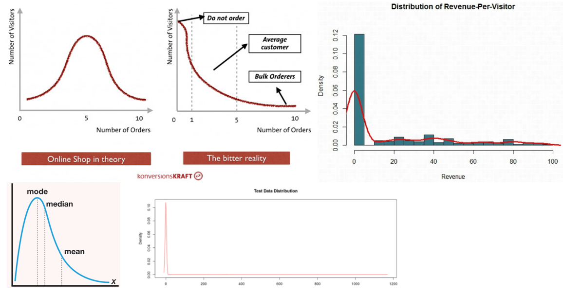
While searching for information on how to calculate statistical significance for revenue-based metrics, one can find at least a couple of examples of blog posts and discussions in which an objection to the use of classical t-tests is raised that is, in short: revenue-based metrics do not follow a normal distribution, thus classical tests are not appropriate. Here are some graphs that are used to illustrate this point:

Many of them make the correct observation that in the case of measuring average revenue per user one needs to essentially account for two types of variance. First – the variance of the conversion rate, that is, did the user order or not. Second – the variance in average order value. The first is known to be binomial, but the second is not. User conversion rate multiplied by the average order value gives us the average revenue per user.

Different alternatives are proposed to handle the issue, like the Mann-Whitney-Wilcoxon rank-sum test, methods from so-called robust statistics, as well as bootstrapping resampling methods. These approaches are fairly complex and while they make less or no assumptions about the distribution, they are much more difficult to interpret. While they have their place and time, I don’t think their introduction is necessary for dealing with non-binomial metrics in A/B testing.

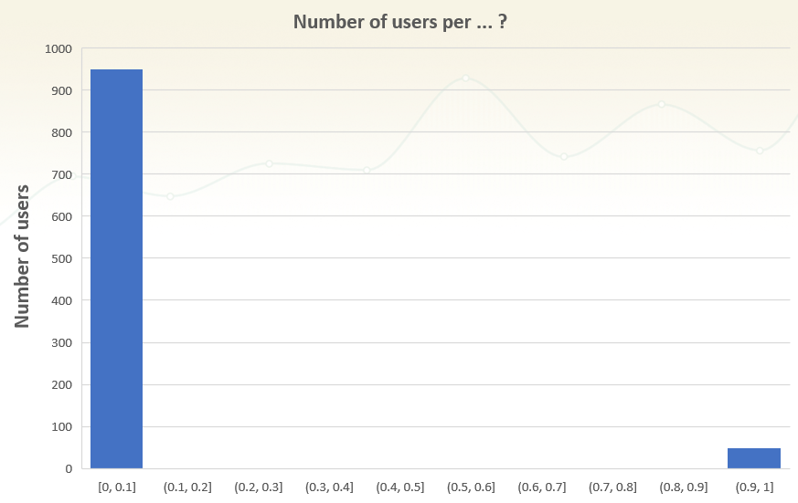
Let me illustrate why by first bringing to your attention the following graph of a well-known family of metrics:

Can you recognize the distribution of which metric has the above shape?

If you guessed correctly, then yes, this can be any rate-based metric, such as add to cart conversion rate, e-commerce transaction conversion rate, bounce rate, etc. So, it doesn’t have a normal distribution, but why is it justified to use classic tests that assume normality?

The reason is simple:

it is the sample statistic error distribution that matters, not the sample data distribution

Sample what? OK, let me explain…

In-sample data distribution vs. sample statistic error distribution

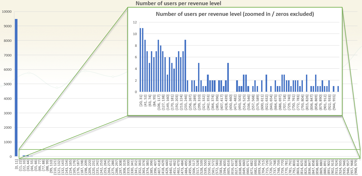
Here is a simulated revenue per user distribution:

(click for large version)

The above is revenue data from 10,000 simulated users. On the x-axis is the revenue bucket, on the y-axis: how many users are in each bucket. It is just like the graphs cited above: the distribution is extremely heavily skewed to the left, since the vast majority of users don’t purchase anything. About 5% of users purchased something.

Looking at the zoomed-in graph, where 0-revenue users are excluded, it is obvious that they are, too, skewed to the left. Much more users place orders in the 20-200 range than in the 200-1000 range. The particular distribution will vary depending on the type of business – online shops selling small items versus ones that sell high-value products will have very different distributions. SaaS businesses will have data that is concentrated around specific revenue levels, corresponding to the tiers they offer. That is beyond the point, though, the data is certainly representative of a vast array of real-world scenarios and the in-sample data distribution is certainly non-normal.

However, significance calculations deal with sample statistics, not with individual data points. Some possible statistics in this case are: the data mean, median and mode. The average is typically used as the most actionable statistic, but the median can also be useful if the goal is to learn the transaction revenue that is paid by the highest number of our visitors. A median shows how much is paid, at most, by half of the visitors. The mean in this case is $10.02. So, if there are two such samples, one with a mean 10.02 and another with a mean of 10.3, a statistical significance test would measure the difference between these two values, not the difference between each and every individual user.

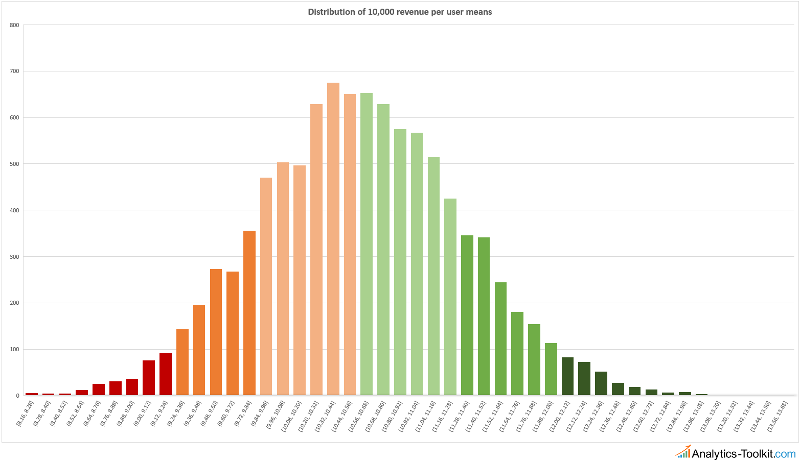
This means that the normality requirement, or assumption, needs to hold for the distribution of the sample statistic, and not for the distribution of the in-sample data shown here. In other words, the interesting variable is the distribution of the error of the mean, not the data itself. In order to check the normality assumption, I generated 10,000 simulations with 10,000 users in each, recorded their mean and plotted it as a histogram. The x-axis is the average revenue per user range, while the y-axis is how many of the simulations ended up in that range, out of the total of 10,000.

(click for large version)

Since all revenue values generated were random, the above plot illustrates the random error of the mean that would be inherent to any measurement of average revenue per user. This is how the noise in your data is shaped, which is what you need to compensate for before you can extract the signal. And its distribution is quite close to a normal curve. Of course, it is impossible to get a true normal curve with just 10,000 simulations, but the important thing is that the more simulations are run, the more the values would converge to a true normal distribution. This asymptotic convergence is what makes statistical tools work.

In other words, the Central Limit Theorem still holds, so there is no need to use more or less exotic tools to work with continuous metrics like revenue per user, average order value, average time on site and the like. However, just because the issue highlighted as central on most blog posts discussing this topic is not present doesn’t automatically mean that you can just use a calculator that only works with binomial data to calculate statistical significance and confidence intervals for non-binomial data.

Calculating significance for non-binomial metrics in A/B testing

Now that it has been demonstrated that there is no need to worry about the normal distribution of our non-binomial metrics, what is holding us back from using just any significance calculators, same as would be done for a conversion rate metric?

The unknown variance of the sample mean makes it impossible to use calculators that work fine with binomial data.

The variance of the sample mean can be calculated easily through a mathematical formula based on the proportion of observations in each sample and the total observations in the tested variants and control. However, for revenue and other non-binomial metrics one needs to estimate the variance from the sample, before calculating significance. The process is fairly straightforward and looks like so:

• Extract user-level data (orders, revenue) or session-level data (session duration, pages per session) or order-level data (revenue, number of items) for the control and the variant
• Calculate the sample standard deviation of each
• Calculate the pooled standard error of the mean
• Use the SEM in any significance calculator / software that supports the specification of SEM in calculations

Different software will have different procedures for exacting user-level or session-level data. In Google Analytics you can use the user explorer report through an API tool, or a custom dimension that contains a user-ID (you can use the Google Analytics Client-ID for non-logged in users). The important thing to remember is that you need to end up with a table in which you have individual users/sessions/orders in one row, and the revenue (or another metric) for that particular user/session/order.

1. Estimating variance from a sample

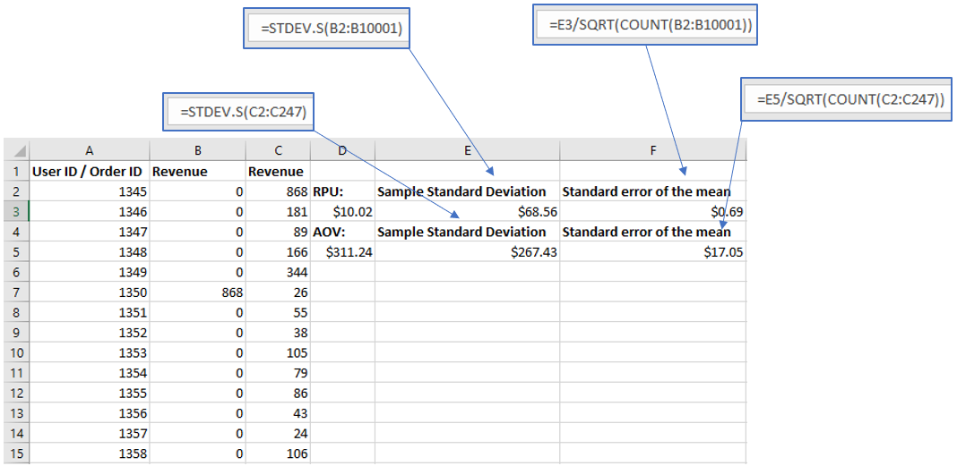
Once you have above, the calculation is simple. You can do in Excel with a few fairly simple formulas:

So, the standard error of the mean revenue per user is estimated at $0.69 from that sample. If you look at the graph for the simulated distribution of the means you will notice that the standard deviation of the mean is estimated at $0.73 from those 10,000 simulated means. Pretty close, meaning the estimate drawn from that one sample was a pretty good estimate indeed. If you notice the coloring of the graph, it corresponds to standard deviations in either direction. The 97.5% one-sided significance corresponds roughly to where the dark green area begins. Another way is to use an online tool, such as this standard deviation calculator, which conveniently also calculates the standard error of the mean (SEM).

2. Calculating significance for non-binomial metrics

In order to plan a test that has a non-binomial metric as a primary KPI you need to estimate the variance from historical data. The more – the better, but I’d suggest to not go too far back, maybe no more than a year since older data might have less predictive value than newer data due to changes in user behavior. The procedure described above should be used.

After a test is ended, you calculate SEM for all variants and the control, you can use any calculator or software tool that supports non-binomial metrics, that is, any t-test calculator that allows you to enter a standard deviation for the mean. What happens is that the pooled variance is calculated, using the combined data of all tested variants and the control, then the t-value and corresponding p-value is calculated using standard approaches. I believe the pooled variance from the test itself will have better predictive value than historical data and should therefore be preferred.

See this in action

Try itStatistical Significance Calculator
Robust p-value and confidence interval calculation.

As with any other statistical significance calculation, you should not be peeking at your data or using reaching statistical significance as a stopping rule unless you are using a proper sequential testing methodology, for example the AGILE A/B testing method.

Calculator for revenue-based and other non-binomial metrics

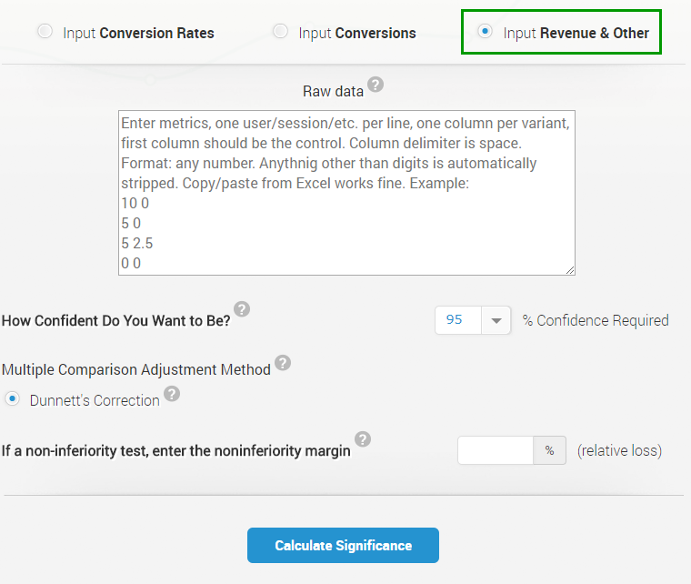
While there are multiple ways to calculate such data, including in Excel or R, we got feedback that it would be a convenience to have all of these automated, so that the process is streamlined and faster to perform. Thus, we have just released an online calculator that allows you to copy/paste data for tens of thousands of lines of user-level, order-level, or session-level data, and it does all calculations automatically, outputting the corresponding p-value and confidence intervals for each variant. The p-values are adjusted for multiple comparisons using the Dunnett’s method. You can try it for free by signing up for Analytics-Toolkit.com and going to our statistical significance calculator, where you should choose to input Revenue & Other data.

Our statistical calculators now also offer the ability to estimate the required sample size when comparing means (difference of means), so now you have all basic tooling necessary to perform the statistical design and evaluation for a simple fixed sample size test with non-binomial data. It has support for tests with more than one variant vs. a control in the case of revenue, AOV, ToS and other such metrics. It uses the Dunnett’s correction to assure control of the Family-Wise Error Rate.

See this in action

Try itA/B Testing Calculator
Advanced significance & confidence interval calculator.

About the author

Georgi Georgiev

Managing owner of Web Focus and creator of Analytics-toolkit.com, Georgi has over twenty years of experience in online marketing, web analytics, statistics, and design of business experiments for hundreds of websites.

He is the author of the book "Statistical Methods in Online A/B Testing", of white papers on statistical analysis of A/B tests, and has been a speaker at conferences, seminars, and courses. Georgi has been distinguished as a winner in the Data & Analytics category of the 2024 Experimentation Thought Leadership Awards.