Futility Stopping Rules in AGILE A/B Testing

In this article we continue our examination of the AGILE statistical approach to AB testing with a more in-depth look into futility stopping, or stopping early for lack of positive effect (lack of superiority). We’ll cover why such rules are helpful and how they help boost the ROI of A/B testing, why a rigorous statistical rule is required in order to stop early when results are unpromising or negative and how it works in practice. We’re reviewing this from the standpoint of the AGILE method (white paper available here) and our AGILE AB Testing statistical calculator in particular.

Why Would We Want to Stop Early for Lack of Effect?

It’s fairly obvious why one would want a rule for early stopping for futility, but let’s lay it out just for completeness. First of all, it’s clear that ideally we want each of our tests to result in significant gains/lift, no matter if we’re testing a shopping cart, a landing page, e-mail template or ad copy. However, that is not always the case, especially when we are trying to optimize and already optimized process, page, template or ad copy.

Stopping an A/B or MVT test early when the data suggests a very low probability that any of the tested variants is going to prove superior to the control is useful since it allows us to fail fast. This means we can:

• stop sending traffic to variations which are no better or even worse than the control, which means we don’t lose as many conversions as if we continue the test
• stop expending resources to QA, analyze, report on, have meetings, etc. for a test which is unlikely to pay off these investments
• start our next test earlier and divert resources from the unpromising test to a potentially more promising one

In essence, when stopping early for futility we usually infer that if we have continued to run the test with more users, there is a very slim probability that we’ll detect a statistically significant discrepancy of a specified size. As always, what “low probability” is and consequently – what the stopping for futility level is can vary greatly from test to test.

Without a rigorous statistical rule to guide our decision, we are likely to succumb to the temptation to stop early when initial results look bad, with an arbitrarily high probability that we’re in fact failing to discover a genuine effect from our treatments. This is called a “type II error” and without a rule we have an unknown probability of committing it. With a statistically-rigorous rule for stopping we know what our probability to commit a type II error. Usually it is expressed as a stopping boundary which serves as a bound to the amount of such error that is admissible in our particular test.

Here is how it would look like if a futility boundary is crossed:

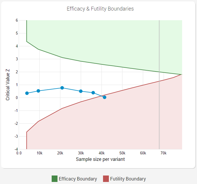
As can be seen from the graph when using the AGILE statistical method, one can have a very flexible monitoring schedule (number and timing of interim analyses) and still maintain proper error control.

Efficiency Gains from Adding a Futility Stopping Rule to an A/B Test Design

Here is a test with designated 5% statistical significance level and 90% statistical power to detect a 10% relative lift from a baseline of 1.5%, with just an efficacy stopping boundary planned for 12 analyses:

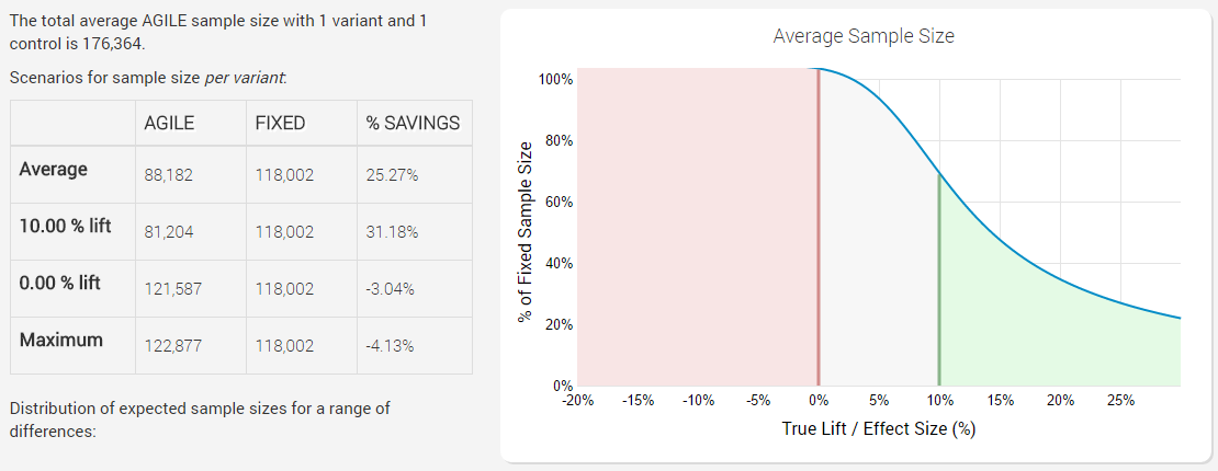
The x axis of the graph has different possible true effect sizes (percent points lift), while the y axes shows sample size (number of users) as percentage of fixed sample size. The higher the percentage – the more users you would need to run the test with, to reach the same conclusion with the same error guarantees, meaning a higher percentage there is equivalent to a less-efficient test.

We can easily see that introducing an efficacy stopping boundary results in significant savings on average: 25.27%, which comes entirely from cases when there is in fact a true positive lift. Bear in mind that this average is under a distribution of true values which is skewed towards positive lifts (the range is +-1 from our minimum effect size of 0.5, which is from -0.5 p.p. to + 1.5 p.p.). If the test performs much better than the minimum effect size, the savings are very significant: for example, if the true lift is 30% having an efficacy stopping boundary will mean we’ll run the test with only 20% of an equivalent fixed-horizon test (that’s a whopping 80% less users!).

However, if the lift is exactly 0%, then we will in fact need about 3% more users compared to a fixed-horizon test, which is due to the sample-size compensation for peeking during the test. In the worst case where the test runs to it’s end we’d need about 4% more users! So we gain a lot of efficiency when the results are positive, but we are certain to lose efficiency when the true performance of the tested variant is null or negative.

Now, let’s introduce the futility boundary and see what happens. Here is the same test (5% statistical significance level, 90% power to detect a 10% lift from a baseline of 1.5%), but this time with an efficacy stopping boundary and a non-binding (we’ll get to that below) futility stopping boundary planned for 12 analyses:

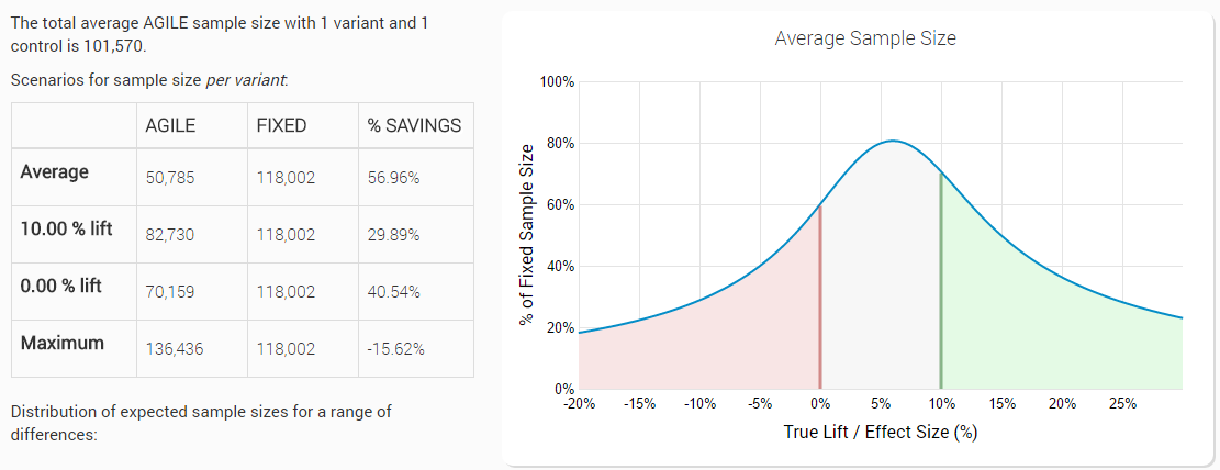
We can easily see that introducing a futility stopping boundary in addition to the efficacy stopping boundary resulted in significant reduction of the expected number of users: 56.96% on average. This is a gain of 125% in average efficiency compared to having just an efficacy stopping rule!

Bear in mind that this average is again under a distribution of true values which is skewed towards positive lifts (the range is from -20% lift to +30%), so if you in fact happen to run many tests with null or negative true lift (e.g. in late-stage testing an already very well optimized landing page/shopping process/e-mail template) the actual performance gains can be significantly higher!

This improved efficiency comes entirely from cases when the lift is less than the minimum lift we’re interested in detecting. As you can see the graph slopes down around the 6% point on the x axis and the smaller the % on the y axis, the more efficient the test is.  The expected average efficiency is worst with true values just under the minimum detectable effect and the graph is asymmetric due to the slightly different spending functions used for efficacy and futility (Kim & DeMets power functions with upper boundaries of 2 for futility (beta-spending) and 3 for efficacy (alpha-spending)).

If the test performs much worse than the minimum effect size, the savings easily reach 75% if the true lift is a negative 11%, meaning we’d be able to run the test with only 25% of an equivalent fixed-horizon test, and with even more savings if compared to a design with stopping rules only for efficacy.

Of course, everything is a compromise in designing an A/B test and having a futility stopping rule has its cost as well. In the worst case scenario, we may end up running the test with as many as 15.62% of the users that a fixed sample-size test would have required. However, applying combined efficacy & futility stopping to a series of tests we are likely to be able to run them with significantly improved efficiency and thus ROI.

On the Statistics Behind Rigorous Early Stopping for Futility

In AB testing the sensitivity of the test is expressed by it’s power. The more powerful a test, the more sensitive it is, that is – the more likely it is to detect a given discrepancy at a specified statistical significance level. A decision to stop early cannot be made while also maintaining the sensitivity of the test to the specified minimum effect size, unless using a statistically justified futility boundary.

Since futility stopping is based on the power of a test, it’s important to understand how to choose a proper power level. Choosing a satisfactory power level is as important as choosing the significance level and the effect size, but sometimes underestimated in practice. The more powerful the test, the more likely one is to detect an improvement of a given size with a specified level of certainty (if such exists in reality). Thus the greater the sensitivity of the test, the bigger the sample size required, or we can say that power is positively correlated with the number of users a test will require.

The decision on the power of the test should be informed by the potential losses of missing a true effect of the specified size, the difficulty and costs involved in preparing the test and how costly it is to commit x% more users into the test. If the test preparation is long and difficult or if increasing the sample size is cheap then we should generally aim for a more powerful test. Note that increasing both power and the statistical significance level result in committing more users to a test, so a balance between the two must be sought.

In the AGILE method for A/B testing we use a so-called beta-spending approach, based on the work of Pampallona et al. (2001) ^[4], who extended the alpha-spending approach of Lan and DeMets (1983) ^[2,3] to the construction of futility boundaries for early termination of the experiment in favor of the null hypothesis. Of course, it happens under the constraints of the test – minimum detectable size, significance level and power. What beta-spending means is that we define a function to allocate type II error depending on how early or late in the test we are. Generally, error-spending functions allocate more error towards the end of a test, where it is best utilized and the results are most informative.

The method used by default for the construction of the futility boundary in our calculator uses a Kim & DeMets (1987) ^[1] power function with an upper boundary of 2. It is less conservative than the one employed for the efficacy boundary, but is still significantly more conservative than, for example, the Pocock-type bounds which are at the other extreme.

Because introducing stopping for futility decreases the overall power and increases the type II error of the test, sample size adjustments are made in order to preserve the power and thus keep the false negative rate at the desired level. Consequentially, designs with a futility boundary require a larger amount of observations if the test is continued to its end, however, they offer a significant improvement to the average expected sample size due to the ability to stop early when the results are highly unpromising or negative.

Binding versus Non-Binding Futility Boundaries

There are two types of futility boundaries a statistical practitioner can choose from – binding and non-binding. With a binding boundary one commits to stop the test when the observed statistic crossed the futility boundary. Failure to do so would lead to an unaccounted for increase in the type I error of the test. Since having a futility boundary means that there is now chance that we’ll stop the trial in favor of the null hypothesis, this decreases the level of alpha or type I error. To keep the statistical significance at the required level we adjust the efficacy boundaries so they are now lower on the Z scale compared to a design with stopping just for efficacy.

With non-binding futility boundary, a crossing of the boundary serves more as a guideline than as a strict rule. One is free to decide whether to stop the test or not, based on external information or considerations, without affecting the level of type I error since the boundary is constructed separately from the efficacy one.

Introducing a binding or a non-binding futility stopping leads to a decrease in power, which is compensated for by an increase in sample size so that we can maintain the desired type II level. The non-binding approach is costlier in terms of sample size, however, that is offset by the gained flexibility under certain conditions. The increased flexibility to consider external factors is the reason why non-binding stopping rules are generally recommended.

See this in action

Try itA/B Testing Calculator
Advanced significance & confidence interval calculator.

Lets use an example to illustrate what the trade-off might look like and why we generally go for a non-binding futility boundary. Taking the same test as above: 5% statistical significance level, 90% power to detect a 10% relative lift from a 1.5% baseline, 12 planned analyses, with a non-binding futility boundary have the following efficiency characteristics:

While a test with a binding boundary has the following design characteristics:

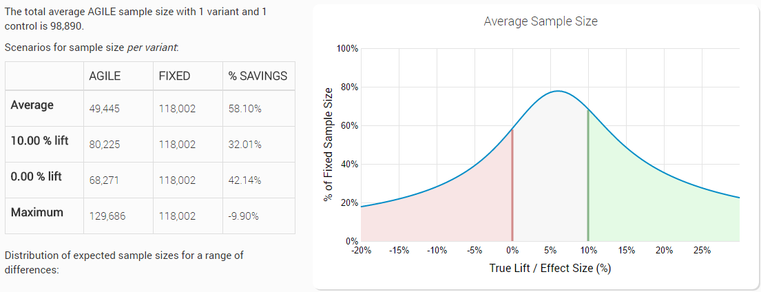
We can see that we’ve gained 1.14 percent points average efficiency and have decreased the loss in the worst-case sample size from 15.62% to 9.90% (vs a fixed horizon test). What we argue is that the fairly modest gains in efficiency cannot offset the strict requirement to stop the test, even if outside considerations might require otherwise. In medical settings the DMCA regulatory body requires non-binding futility bounds as well. However, we do allow users to choose between the two, based on their particular preferences.

Concluding Remarks

It is evident that stopping early for lack of positive effect is essential in improving the return on investment from A/B testing in any setting. The approaches used to control type I and type II errors are statistically rigorous and proven in their use in medical research in the past decades. The efficiency gains of over 55% compared to fixed-sample tests and the doubling of the efficiency when compared to tests with rules for stopping only for efficacy make the use of futility stopping a near-requirement for nearly every statistical design in A/B test.

To learn more about efficient A/B testing, read our AGILE A/B Testing whitepaper or try our A/B Testing Calculator.

References

1 Kim, K., DeMets, D.L. (1987) “Design and Analysis of Group Sequential Tests Based on Type I Error Spending Rate Functions”, Biometrika 74:149-154.
2 Lan, K.K.G, DeMets, D.L (1983) “Discrete Sequential Boundaries for Clinical Trials”, Biometrika 70:659-663
3 Lan, K.K.G, DeMets, D.L (1994) “Interim Analysis: The Alpha Spending Function Approach”, Statistics in Medicine 13:1341-52
4 Pampallona, S., Tsiatis, A.A., Kim, K.M. (2001) “Interim Monitoring of Group Sequential Trials Using Spending Functions for the Type I and Type II Error Probabilities”, Drug Information Journal 35:1113-1121

About the author