Using Observed Power in Online A/B Tests

Observed power, often referred to as “post hoc power” and “retrospective power” is the statistical power of a test to detect a true effect equal to the observed effect size. “Detect” in the context of a statistical hypothesis test means to result in a statistically significant outcome.

Some calculators aimed at A/B testing practitioners use observed power to guide users as to what the sample size of their test should be. When performing statistical significance calculations, these tools present something like “Required sample size” or “How long to run the test for” next to their results. Those numbers are apparently supposed to tell if the test needs to run for longer or not, or at the very least to indicate if a test is underpowered or overpowered.

Despite several attempts over the years to nudge the authors of said tools to remove this harmful “functionality” from their calculators, it continues to exist. Given the relative popularity of these tools among less experienced practitioners, the use of observed power may be doing noticeable harm to the online experimentation field, hence this article.

The following topics are covered below:

1. Using observed power in practice
2. Requiring statistical significance AND high observed power
3. Fishing for high observed power
   3.1 The simulation
   3.2 Results from peeking through observed power
4. Takeaways

Using observed power in practice

There are three possible scenarios for using observed power in any one of these calculators:

1. The outcome of an A/B test is calculated as being statistically significant, and the observed power is higher than whatever threshold was chosen (80%, 90%, etc.). In this case the calculator will almost always say that the test was overpowered. In other words, one has “waited for too long” and has exposed too many users to the test. For example, the sample size may have been 10,000 users per variant, but the “Required sample size” field may say only 8,000 were needed.
   
2. The outcome may be statistically significant, but the observed power is lower than the chosen threshold, which will (wrongly) suggest the test was underpowered. One might interpret this to mean the test is untrustworthy and cause them to ignore a perfectly valid statistically significant outcome. A different interpretation may be to treat the low observed power as a license to continue the test at least until the “Required sample size” is reached and perhaps even for longer if it happens to need even more data after that first extension. Both of these routes lead to very different outcomes.
   
3. Finally, the outcome may not be statistically significant, in which case the calculator will always suggest the A/B test is significantly underpowered. For example, a user may have tested with 10,000 users per variant, but the “Required sample size” output will inform them they need multiple times larger sample size, with numbers 5x or 10x not being uncommon. In the same example that would mean the tools suggest exposing 40,000 or 90,000 more users per variant than had initially been planned (assuming there was a plan) and taking five to ten times longer.

Notably, one is almost never going to see that their test is well-powered based on observed power calculations. The math is bound to almost always label an A/B test as either underpowered (more often), or overpowered (typically less often). My comprehensive guide on observed power would be a great read for anyone keen on understanding the matter in detail, and it explains why the above scenarios encapsulate all that can happen. It also includes a calculator which lets you thoroughly explore observed power.

In the first scenario many experimenters would typically just walk away with a statistically significant finding. What happens in each of the other two scenarios is far more interesting. Let us deal with them one by one.

Requiring statistical significance AND high observed power

In scenario two some practitioners will just ignore the warning about their test “requiring more users” or “more time” since the result is statistically significant. However, some might be swayed into accepting a test’s significant outcome only if the outcome is both statistically significant and “well-powered” or “overpowered” (based on observed power). This kind of behavior leads to multiple times more stringent type I error control than the nominal threshold sets.

The exact type I error which would be achieved can be estimated easily by plotting p-values and observed power on a graph, and checking what p-value corresponds to the chosen power level. This can also be done with the post hoc power calculator I’ve created for educational purposes.

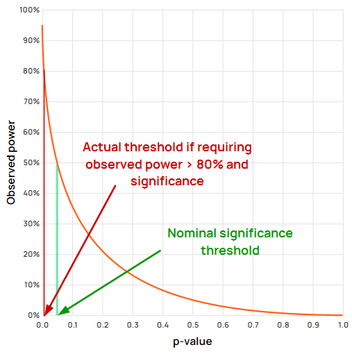
For example, using “textbook” values of 0.05 and 0.80 as the cut-off for significance and for observed power (80% power of the design), one would in fact achieve a type I error rate of about 0.6%, or more than eight times smaller than the target 5%. Note that the same is true if one requires the observed effect to be greater than the MDE.

If using 0.05 significance threshold and 90% power, the actual type I error rate would be 0.17%, or about thirty times smaller than the target of 5%. If using a stricter significance threshold of 0.01 with 80% power, the actual type I rate is 0.076%, or about thirteen times smaller, and so on. The stricter each of the thresholds is, the smaller the actual type I error attained through this approach.

Additionally I have confirmed all of the above independently through simulations.

Such a practice has a crippling effect on the achieved statistical power, which instead of being 80% or 90%, is reduced significantly. If it is not obvious why that is a big issue, consider The importance of statistical power in online A/B testing.

A different problem faces those who might choose to continue the initially significant but seemingly underpowered test until it is eventually both statistically significant and well-powered. Interestingly, my simulations show that such A/B tests will not suffer from an inflation of their type I error. However, they should expect to commit to an eightfold increase in sample size, on average, at least in the cases where there is no true effect or it is of minimal size.

Fishing for high observed power

In scenario three, some may interpret the fact that their sample size is many times lower than the “required sample size” as a license to continue testing until the recommended sample size is reached. After all, if a statistically insignificant test seems “underpowered”, it sounds like there is a true effect waiting to be found, if one just extends their sample size to what’s needed to make it “powerful enough”. Why then not to continue testing for however long it takes to reach the “required sample size” suggested by the calculator?

However, examining A/B test data with an intent to stop based on the outcome constitutes peeking and is a violation of crucial assumptions behind the tests used in these calculators. Classic peeking is sometimes called “fishing for significance” so by analogy we may call this approach “fishing for observed power”. Just like its cousin, peeking through observed power results in an inflated false positive rate (type I error rate). In a typical scenario of a one-sided test, if the true effect is zero or negative, statistically significant outcomes would be “found” multiple times more often than the nominal p-value or confidence level would suggest.

Unlike classic peeking, how much type I error inflation one is bound to get by fishing for high observed power is unknown, at least as far as I am aware. Given this, a simulation is a straightforward way to emulate the behavior of peeking through observed power and to estimate what it leads to.

The simulation

The simulation below was performed under the following assumptions:

• one starts with some reasonable sample size before their first calculation of observed power
• one stops a test immediately if it is nominally statistically significant at any evaluation (regardless of post hoc power)
• if the observed effect is zero or negative, the test stops (it will be non-significant)
• if the observed effect is positive, the test is extended with the recommended sample size calculated using the observed effect size as an MDE, but the extension is truncated to no more than 10 times the initial sample size. Changing this parameter or removing it altogether does not meaningfully alter the outcomes, but makes the simulations more tractable and somewhat closer to reality.
• if after one or more extensions the sample size reaches 49 times the initial sample size, the test stops regardless of outcome. This is to keep the simulation somewhat closer to real life where few if any would be willing to continue past such large multiples of the original sample size.

The above describes scenario 3 with some limits added to keep things realistic. What happens without some of those limits is shared in Appendix I as a sanity check.

100,000 simulation runs were performed with the following parameters:

• a true effect of exactly zero
• an initial sample size of 50,000 users per variant
• a significance threshold of 0.05 (textbook value, equivalent to requiring at least 95% confidence), resulting in a target type I error rate of 5%.
• a power threshold of 0.8 (80%) to which observed power was compared and which was used to perform the “required sample size” calculation

The summary results are presented below.

What happens when peeking through observed power

Since observed power and p-values have a direct functional relationship, it is unsurprising that fishing for high observed power is in a way fishing for statistical significance. Expectedly, it results in an inflation of the type I error.

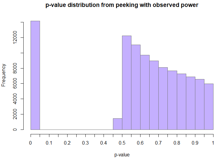
11,685 out of 100,000 simulations resulted in a statistically significant outcome, meaning the type I error rate was 11.685% instead of the target 5%, representing a nearly 2.4x increase of the false positive rate. Additionally, the average sample size these tests ended up with was close to 540,000 users per variant which is more than 10x the initial target of 50,000.

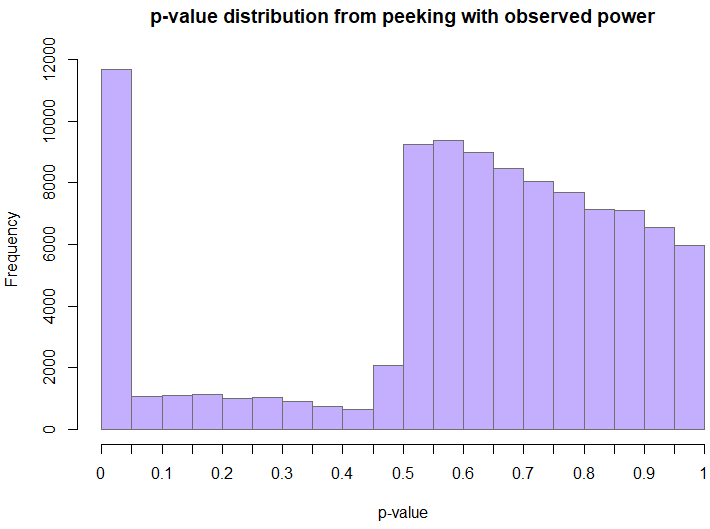
The distribution of p-values is decidedly non-uniform, and highly skewed towards low values (a proper p-value should have a uniform distribution under a true null). The fact that there are any values between 0.05 and 0.5 at all is mostly due to the maximum sample size limit of 49x the initial sample size.

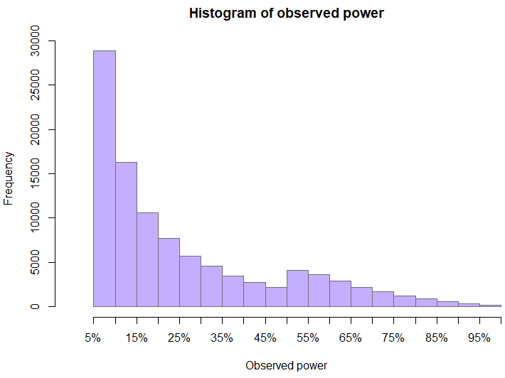
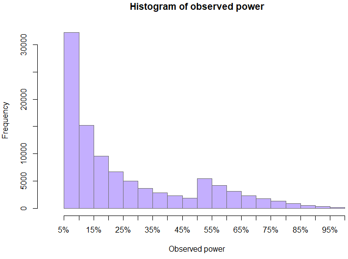
The distribution of observed power at the time when a test was stopped is also somewhat interesting. The skewed nature of the distribution is entirely expected even without peeking, but the bump just above 50% is not. Peeking is what formed the “valley” to the left of 50%. Since values above 50% are those of tests with statistically significant outcomes, it was values that were initially just below 50% which got extended and since the true effect is zero, these tests ended up with a smaller observed power as the observed effect drifts towards the true effects with increasing sample size.

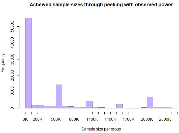
The peculiar nature of the sample size distribution is due to the caps on how much the “required sample size” is allowed to increase the sample size at each step. The higher proportion of achieved sample sizes above 2mln users per variant compared to the earlier segment is due to the maximum cap on the sample size.

Takeaways

Using observed power in any way is harmful to the error control and trustworthiness of any experiment. At the very least, observed power will almost surely label a test as either underpowered or overpowered, without any reference to it’s actual qualities. However, different scenarios of using observed power result in additional problems of severe consequences.

Requiring observed power in conjunction with a statistically significant outcome in order to reject a null hypothesis results in a nominal false positive rate multiple times higher than the one actually achieved. It raises the bar of evidence required to declare a “winning” experiment to levels far above the initially targeted. If one ignores significant outcomes from “underpowered” tests and continues testing until the outcome is both significant and the observed power is above the target power level, then it is just a massive (more than eightfold) waste of time and user exposure.

When observed power is used with non-significant outcomes to guide how long to run a test for and with what sample size, the effect is similar to classic peeking. This practice leads to multiple times higher actual false positive rate versus the nominal one (an inflated type I error rate) with realistic simulations showing this increase to be at least 2.4x. Altering the assumptions more or less generously regarding what a practitioner does results in actual error rates between two times and three times the target error rate. A test with such a discrepancy between its target (or reported) error rate and its actual one cannot be seen as valid or trustworthy.

If you have found the above interesting, you might consider checking out the statistically-rigorous A/B testing calculators at Analytics Toolkit.

---

Appendix I. Simulation results with different caps

1) This first set of results are without the hard limit on the total sample size being no more than 49x the initial sample size after all possible sample size increases.

14,169 out of 100,000 simulations resulted in a statistically significant outcome, meaning the type I error rate was 14.169% instead of the target 5%, representing a more than 2.8x increase of the false positive rate. The average sample size these tests ended up with was close to 1,120,000 users per variant which is more than 22x the initial target of 50,000.

The resulting distributions are:

The sample size distribution is too heavy tailed to feature here in a meaningful manner.

2) Removing both the hard 49x limit and the limit on each increment to be no more than 10x the initial sample size results in a false positive rate of around 12.5% (with a target type I error of 5%).

3) Lowering the limit on each increment from 10x the initial sample size to 2x the initial sample size while retaining the hard 49x limit results in a false positive rate of around 14.5% (again with the nominal level being 5%). The reason is that it results in more peeks than the 10x limit.

About the author