
One topic has surfaced in my ten years of developing statistical tools, consulting, and participating in discussions and conversations with CRO & A/B testing practitioners as causing the most confusion and that is statistical power and the related concept of minimum detectable effect (MDE). Some myths were previously dispelled in “Underpowered A/B tests – confusions, myths, and reality”, “A comprehensive guide to observed power (post hoc power)”, and other works. Yet others remain.
A major reason for the misuse and misunderstanding of statistical power can be found in the textbook approach to designing statistical tests. It has long been exposed as relying too much on a combination of conventions and guesswork. A data-driven approach for designing statistical tests is proposed as a potent alternative. Its focus on achieving an optimal balance of business risk and reward provides context which illuminates the proper role of statistical power in coming up with good A/B test plans.
The content is structured as follows:
- What is statistical power
- The power level of a test
- The minimum effect of interest
- The classic approach to designing statistical tests
- Risk/reward optimization in designing statistical tests
- Minimum detectable effect – redefined?
- The role of an expected effect in A/B testing
- Conclusion
What is statistical power
The power of a statistical test is a function of its sample size and confidence threshold over the range of all possible values of the parameters of interest. Its curve is defined by the probabilities to reject the null hypothesis over all possible values of the parameter of interest.
The statistical power of a test is a function of its sample size and confidence threshold showing the probability to reject the null hypothesis over all possible values of the parameter of interest
The sample size is often a number of users or sessions, the confidence threshold (or significance threshold) defines the limit on the probability of conducting a type I error, while the parameter of interest is the primary performance indicator for the success or failure of the tested change, typically expressed as percentage change (a.k.a. % lift).
If one assumes known variance, the only other parameters which define the power function are the desired confidence threshold and the sample size of the test. Statistical power is a characteristic of the test at hand, as opposed to a parameter that one sets.
Notably, its definition and calculation does not refer to or require an estimate or prediction of:
- what the true effect size is
- what the observed effect would be
- what the minimum effect of interest is
Here is an example power function curve for a test with a sample size of 160,000 users, textbook 95% confidence threshold, and a baseline conversion rate of 2% as displayed in the Analytics Toolkit’s A/B test creation wizard:
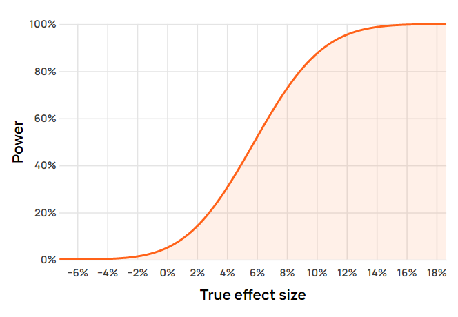
The power curve can be examined at any point on the x-axis to calculate the probability of rejecting the null hypothesis at that particular true value of the parameter of interest. This gives us the power level at that point.
The power level of a test
When one speaks of “statistical power of a test” it typically refers to “the power level at a given effect size of interest” instead of the power function over the entire set of possible parameter values. Separating the two aspects of power calculation and presentation may introduce some clarity.
In the previous section “statistical power” was defined as the function over all possible values of the parameter, hence the definition of a specific power level would be:
The power level of a statistical test is defined as the probability of observing a p-value statistically significant at a certain threshold α if a true effect of a certain magnitude μ1 is in fact present.
The generic formula for the power level of a statistical test at a given true effect size is:
POW(T(α); μ1) = P(d(X) > c(α); μ = μ1)
meaning the power curve can be computed at any possible true effect size μ1 by just knowing the sample size, the estimated variance (in this case obtained analytically through the baseline proportion of 2%), and c(α) – the critical value corresponding to the desired confidence threshold. The latter three fully define T(α). In this example the confidence threshold of 95% translates to a significance threshold of 0.05 which in a one-sided test is achieved at c(α) ~= 1.644 standard deviations from the mean.
Hence the power level is simply the value of the power function at a specific true effect size. For those familiar with type II errors, it is the inverse of a test’s type II error rate (β, beta) at a certain true effect size μ1.
What effect sizes should we be looking up the power level at? How do we determine which effect sizes are of interest and which are not? These key questions are discussed in the next section.
The minimum effect of interest
As shown above, the definition of a power level requires the specification of a true effect for which to compute it, an effect of interest.
A true effect of interest would be any true effect of practical significance, where what is of practical significance depends on considerations of related losses and gains that need to be taken into account. The smallest of all such effect sizes can be referred to as the ‘minimum effect of interest’ (MEI). The power level at that effect size should be of primary concern in planning an A/B test.
Calculating a power level requires the specification of an effect of interest.
The minimum effect of interest is typically known as the minimum detectable effect (MDE), but in this text the term “minimum effect of interest” is introduced instead. The reason is that it better captures the true meaning; is less prone to misinterpretations; rightly puts emphasis on the fact that external considerations need to be taken into account for it to be determined (more on this in the next section). The term MEI and these arguments were first proposed in an extended form in “Statistical methods in online A/B testing” (2019).
In most cases a single true effect size of interest is chosen and the value of the power function at the point is reported. For example, if the minimum effect of interest (MEI) is +10.5% then the value of the power function at that point is ~90%, in other words the power level is ~90%. If, instead, the minimum effect of interest is 5%, the power level of the same statistical test is just ~41%.
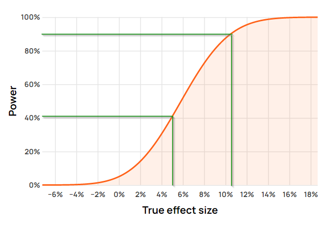
The power level of a test is therefore not just a characteristic of the test. It is determined by the minimum effect of interest which by definition reflects external considerations related to the particular A/B test hypothesis and the business question which informed it.
The classic approach to designing statistical tests
To further illuminate the concepts of statistical power, the power level of a test, and the minimum effect of interest, it is best to examine their role in the process of planning statistical tests.
A textbook view on how to determine the statistical design of a test is adopted from various scientific research applications, mostly in the humanities, including clinical, psychology, and economics experiments. Its prescription is generally to determine the confidence threshold by some convention, then choose a minimum effect of interest at some high power level, again by convention, and finally compute the sample size based on straightforward formulas that take these three parameters as input.
Graphically, it can be presented in this way:
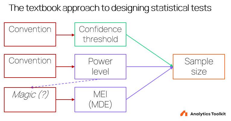
Very rarely one can see arguments for the need to justify these key parameters, even in highly regulated and monitored major clinical trials.
The drawbacks of this approach are immediately apparent:
- The confidence threshold is informed by dubious conventions instead of reflecting the risk of a wrong conclusion which favors replacing the current state of affairs. What convention is chosen may depend on history with scientific experimentation, a perceived average level of risk for all tests, or something else.
- A power level is chosen by convention. It may be less serious of an issue if addressed by altering the MEI/MDE accordingly. Otherwise the same lack of context applies.
- There is an often unrecognized dependency between the power level chosen and the minimum effect of interest. Arguably, one would chose a different MEI if the power level is set at 80% as opposed to 95%.
- There is practically no guidance on how one is to decide on a minimum effect of interest. The best the literature can offer is “It is the difference you would not like to miss” equivalent to no guidance at all without a supporting in-depth discussion.
To justify the strong “magic” wording, here are some citations from the very scant literature relevant to the topic of selecting a minimum effect of interest which is supposed to reflect practical significance:
“In the absence of established standards, the clinical investigator picks what seems like a reasonable value.” [2]
“Given the critical nature of the concept of clinical importance in the design and interpretation of clinical trials, it is of concern that methodological standards have not been developed for determining and reporting the clinical importance of therapies.” [2]
“Statisticians like me think of δ as the difference we would not like to miss and we call this the clinically relevant difference.” [1]
While the above can be a good starting point, no details on how the definition of “clinical relevance” is to be approached in practice are provided.
Symptoms of the impotence of the simple framing like the above reveal themselves in the interpretation of the outcomes as well:
“Authors of RCTs published in major general medical and internal medicine journals do not consistently provide their own interpretation of the clinical importance of their results, and they often do not provide sufficient information to allow readers to make their own interpretation.” [3]
It is no wonder that many A/B testing practitioners when first introduced to the above strategy for planning a test end up saying something like “anything above zero is exciting, so the minimum effect of interest is 0.001%”.
Risk/reward optimization in designing statistical tests
To replace the “magical” approach discussed above, a proper definition of practical significance is called for. Such a definition can be arrived at by taking into account fixed and probability-adjusted benefits and fixed and probability-adjusted costs of running the A/B test. Chapter 11 of “Statistical Methods in Online A/B Testing”: “Optimal significance thresholds and sample sizes”, is dedicated to the logic and math behind the computations.
Only effects for which the benefits outweigh the costs can be called effects of interest. Therefore the minimum effect of interest can be properly defined to be smallest of all such effect sizes.
The above, however, leads to an inconvenient realization which is that a properly calculated minimum effect of interest cannot be defined separately from a test’s sample size. This is true since the practical significance of any true effect is partially a function of the sample size and therefore power of a test, forming a feedback loop. The reason is that the number of people exposed to a test alters both the probability-adjusted losses and gains in a risk/reward calculation. Changing that number affects the missed gains or direct revenue loss both for the duration of the test and post-test, depending on what the true effect of the tested change is.
The thus altered losses and gains then feed back into the calculation of the minimum effect of interest, resulting in a different minimum effect of interest at whatever power level one may choose to examine it at.
The loop is completed by considering that power is also defined by the chosen confidence threshold so any change to that parameter affects the other two. One ends up having to deal with two intertwined feedback loops as shown below:
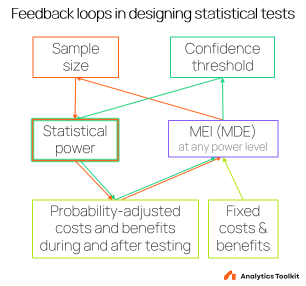
It can be simplified to a single loop in which the sample size and confidence threshold are replaced and the loop leads directly to “Statistical power”, but the above presentation should have greater explanatory power.
The loops involving these parameters make it so complicated to come up with optimal test designs.
The feedback loops involving the minimum effect of interest, the sample size, and the confidence threshold make it complicated to come up with optimal test designs.
Due to these feedback loops, ideally the determination would happen through a risk/reward optimization algorithm. The algorithm presented in the book can be seen in action in the Advanced wizard of the A/B testing hub at Analytics-Toolkit.com.
Absent such a search algorithm, how does one approach the feedback loop? Prioritizing each of the loop components is one way to approach it constructively. First, the initial confidence threshold is defined, then an initial value for the minimum effect of interest is chosen without regard for power, and finally power levels for the MEI at various test durations / sample sizes are examined. The process is then repeated while adjusting all or some of the three variables until the final values of the parameters are arrived at. At that point no further improvement in the balance of risk and reward can be achieved.
Tedious as the above algorithm may be, it is the only way to avoid the alternative that is the textbook amalgam of pure guesswork and ‘conventions’ derived from poor interpretations of statistics works.
Minimum detectable effect, redefined?
The above sections described the planning of a statistical test in the context of online A/B testing without any reference to the term “minimum detectable effect” (MDE). The term “minimum effect of interest” was used as a replacement in that context. However, in a different context, the use of “minimum detectable effect” might remain desirable.
Arguably, it can be used when describing a characteristic of a statistical test at a specified power level of interest. In other words, with an already specified test (in terms of sample size, confidence threshold, and variance) a minimum detectable effect can be obtained at any power level of interest such that:
The minimum detectable effect is the true effect size at which a given test achieves a power level of interest.
In this sense, referring to a minimum detectable effect is equivalent to examining the power function curve from the point of its y-axis, instead of from the point of the x-axis which we have done in the discussion on the minimum effect of interest.
The reason it makes more sense to use MDE in such a scenario is that the power level is explicitly specified, putting context into what “detectable” means and blocking erroneous conclusions such as:
- a test will not produce a statistically significant outcome if the true effect size is less than the MDE at some chosen power level
- if the observed effect size is less than the MDE at some chosen power level, it will not be statistically significant (or if it is, something is wrong with the validity of the test)
The reason we prefer minimum effect of interest in the scenario of planning an A/B test, and minimum detectable effect when examining a test with already specified characteristics and a chosen power level is that however complicated the specification of a minimum effect of interest may be, specifying a power level of interest instead does not fit the typical process of designing A/B tests and likely most experiments in other fields. However, a power level is a requirement for calculating a minimum detectable effect at that level.
From that viewpoint specifying a single power level of interest becomes unnecessary even when the term may see use in test planning. Instead, one can examine a set of several power levels to get an idea of the minimum detectable effect at each, and see how they compare to the MEI. This approach is realized in the “Basic” test creation flow in our A/B testing hub:
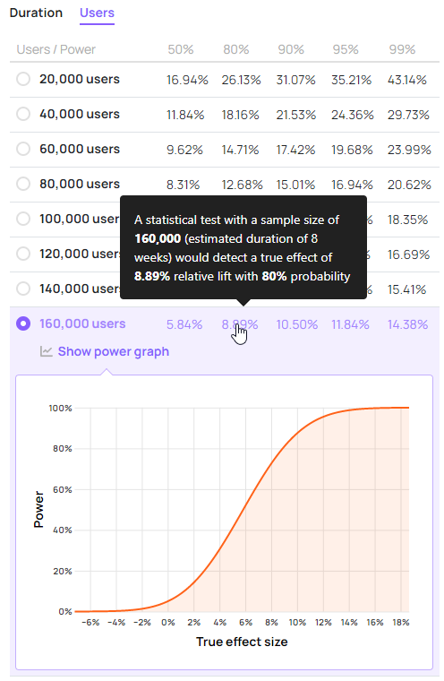
Neither specification of a MEI, nor a power level is needed to generate the table and a power graph for each sample size / duration scenario. However, implicit in the process is the comparison of an effect of interest with the MDEs at different power levels.
The idea of such a presentation is that it allows a practitioner to examine the test power at each sample size / duration scenario. Starting from an initial minimum effect of interest (uninformed by sample size requirements) one can examine the power level at that effect size and/or check how that MEI compares to MDEs presented at certain power levels.
This information can guide a refinement of the size of the initial MEI. For example, an increased test duration aimed at improving power towards the initial MEI changes the balance of probability-adjusted costs and benefits which results in a revised, larger MEI in order to maintain optimal balance of overall risk and reward. This process may need to be repeated a number of times before arriving at a point at which the risk/reward ratio reaches its optima.
Following this process without an automated algorithm is typically impractical due to the involvement of multiple business metrics and integral calculus. Even if one is to do so, it is clear that the minimum effect of interest takes precedence and the minimum detectable effect serves just an auxiliary role.
The role of an expected effect in A/B testing
Expectation, prediction, or estimation of where the true effect size lies plays only a modest role in designing and planning of statistical tests if using the risk/reward optimization approach described above.
It is certainly not the role often mistakenly assigned to such predictions, namely that they should directly translate into the minimum effect of interest. According to this logic, if one expects the true effect from a given intervention to be X% lift, then a test involving said intervention should be planned with a “high” power (say 80% or 90%) towards that effect size. It equates the minimum effect of interest with the expected effect and a given power level. How sound is that logic, though?
Assume the expected true effect of a given proposed change is 10.5% . The 10.5% number is not just a hunch or a wild guess, but the result is well-researched hypotheses, tested on 10 other similar websites, with similar implementation in each case.
Further assume a risk/reward calculation which takes into account a distribution of the expected true effect size outputs that just a 2% true lift is enough to justify both the fixed and probability-adjusted costs. Why should then 10.5% be the minimum effect of interest for which to seek high power, and not 2%? A test with 90% power level against a true effect of 10% means it would have a power level of about 14% against a true effect of 2%.
Why should a business risk running a test with 86% (100%-14%) probability of not detecting a practically significant lift of 2% just because the expected true effect is 10.5%? The 2% lift achieves optimal balance of risk and reward and should therefore be the minimum effect of interest for the test, regardless of any expected true effects greater than 2% such as 10.5%. Running a test with just 14% power against an effect determined to be practically significant in the way described above is unlikely to be wise.
On the other hand, it is also possible that a risk/reward calculation reveals that if one has sufficiently high-confidence prior expectations, running a test would in fact result in a risk-adjusted loss, resulting in the conclusion that one should simply implement. Obviously, such high confidence is not typically realistic, considering all the ancillary hypotheses involved, but it is worth mentioning that the scenario could hypothetically exist.
How likely any of the above situations are to occur under realistic conditions is unclear. It also cannot be said how likely it is that the expected true effect size and the minimum effect of interest would be close to or coincide for a given statistical test. A dozen scenarios run showed an array of possible relationships, and in neither one was the minimum effect of interest equal to the expected lift, but these are more anecdotal accounts than data.
For an example of the significant difference between the minimum effects of interest in two very similar experiments one can look at the COVID vaccine trials run by Pfizer-BioNTech and Moderna (lessons from these for A/B testing discussed at length here). At the same 80% power level, BioNTech’s minimum detectable effect size was 30% while Moderna’s was 60%, or twice larger, despite both companies coming up with and identical solution from a practical standpoint. Why is that? Did both companies really expect their product to result in an effect around 30% and 60% respectively? Were the ~95% observed effect sizes really not anticipated, given that these are Phase III trials?
Both of the above are unlikely. The external considerations taken into account likely included:
- the minimum regulatory requirement for market release of 30%
- the resources needed to conduct the trials. BioNTech with the backing of Pfizer had a much larger budget behind them so that likely factored into their decision to recruit the 43% more participants required for their chosen minimum effect of interest. Moderna, on the other hand, relied heavily on grant money from US government agencies and could only go as far.
- Pfizer-BioNTech spending their own money opting for a lower MEI so that they would get a return on their huge investment even if Phase III results do not meet their expectations, while the same might not have been true for Moderna who spent taxpayer money.
The above are obviously nothing more than informed speculation as I have no insight into how the particular decisions were made and surely do not exhaust the entirety of the factors taken into account for such huge projects.
Conclusion
The article introduces statistical power as a function over the whole set of possible parameter values instead of viewing it as a single, fixed characteristic of a test. It complements that with an understanding of the power level of a test as only specified at a given minimum effect of interest, making the two-way interaction between these concepts explicit which exposes deficiencies in the textbook approach to designing statistical tests.
The discussion on the choice of a minimum effect of interest includes a comparison of said textbook approach with its conventions, guesswork, and “magic” to a risk/reward optimization approach based on sound decision theory. In such a framework the minimum effect of interest at any given power level is where risk and reward trade-offs reach an optimal point, meaning their ratio cannot be improved any further.
The complicated interplay between the variables involved in planning an A/B test using risk/reward optimization and the feedback loops in determining a test’s confidence threshold, minimum effect of interest, and sample size are made explicit. No non-algorithmic solution exists to allow one to design optimal tests in view of said feedback loops. Since the required computations are impractical to do by hand, the use of automated execution of the algorithm is highly recommended.
The term minimum detectable effect is restricted to scenarios when examining the power property of an already defined test is interesting at specific power levels. It should prevent most confusions that arise when used in planning of statistical tests and leaves room for the term MDE in situations where an “effect of interest” is not necessarily relevant or defined.
Finally, the possible confusion between the expected effect size of a proposed change with the minimum effect of interest in planning a statistical test is addressed. While the expected effect size has an influence on the minimum effect size of interest, this influence is in practice limited due to the typically low certainty associated with any prediction given the significant number of assumptions and ancillary hypotheses that need to be taken into account.
Acknowledgements
I’d like to acknowledge Jakub Linowski from GoodUI for the thoughtful feedback and comments on earlier versions of this article which contributed for a clearer and more streamlined presentation. I am to be solely responsible for any remaining errors, omissions, or lack of clarity the reader might encounter.
References:
1 Senn, S. (2014) “Delta Force: To what extent is clinical relevance relevant?”, online at https://errorstatistics.com/2014/03/17/stephen-senn-on-how-to-interpret-discrepancies-against-which-a-test-has-high-power-guest-post/
2 Man-Son-Hing M. et al. (2002) “Determination of the Clinical Importance of Study Results”, Journal of General Internal Medicine, 17(6): 469–476; DOI: 10.1046/j.1525-1497.2002.11111.x
3 Chan K. B. Y. et al. (2001) “How well is the clinical importance of study results reported? An assessment of randomized controlled trials”, Canadian Medical Association Journal, 165(9): 1197–1202
About the author

Managing owner of Web Focus and creator of Analytics-toolkit.com, Georgi has over twenty years of experience in online marketing, web analytics, statistics, and design of business experiments for hundreds of websites.
He is the author of the book "Statistical Methods in Online A/B Testing", of white papers on statistical analysis of A/B tests, and has been a speaker at conferences, seminars, and courses. Georgi has been distinguished as a winner in the Data & Analytics category of the 2024 Experimentation Thought Leadership Awards.

