
Don’t we all want to run tests as quickly as possible, reaching results as conclusive and as certain as possible? Don’t we all want to minimize the number of users we send to an inferior variant and to implement a variant with positive lift as quickly as possible? Don’t we all want to get rid of the illusory results that fail to materialize in the business’ bottom-line?
Of course, we all do, and this is the motivation behind the AGILE A/B testing method we at Analytics-Toolkit.com have developed in order to satisfy the demand for accurate, flexible and most of all efficient solutions. An AGILE A/B test reaches conclusions 20% to 80% faster than the classical methods and solutions while providing the same or better statistical guarantees and significant flexibility in monitoring and acting on data as it accrues.
In this post we explain how A/B or multivariate tests following the AGILE approach work and how using them one can enjoy efficiency and flexibility without compromises with accuracy. Below we cover the basic flow of an A/B test and offer detailed practical advise on how to properly select the different test design parameters. Since no two tests are the same, there is no “best” or “optimal” set of parameters, so don’t skim through the test expecting to find the “secret formula”.
Also available is a white paper describing the whole approach in detail, as well as our statistical calculator for A/B testing which helps automate the most cumbersome parts of the design and analysis of AGILE tests.

9 Steps of Performing an AGILE A/B Test
As any other approach to testing AGILE has two stages: design stage and execution/analysis stage. Test design precedes the launch of the experiment and is where the design parameters are decided on. Analysis happens during the test and also post-test, with some statistics available only after the test is completed.
The application of the AGILE AB testing method can be written as a 9-step procedure with the following steps:
- Decide on the primary design parameters of the test – minimum effect of interest, statistical confidence required, power of the test.
- Decide on the secondary design parameters of the test – number of interim analysis, type of futility boundary (binding vs non-binding), number of tested variations.
- Evaluate the properties of the test design and decide on if it is practically feasible to run the experiment. Adjust the parameters accordingly, accounting for the trade-offs between the parameters.
- Extract data for interim analysis on stages. Can be on a daily/weekly schedule or ad-hoc, or a combination of both.
- A standardized Z test statistic is calculated for the currently best performing variant.
- If there is more than one variant tested against the control, the test statistic is adjusted for family-wise error rate.
- Evaluate the resulting statistic at the latest stage (observation) against the boundaries:
– If the statistic falls within the boundaries, it is suggested that the test continues
– If the efficacy boundary is crossed, consider stopping the test and declaring a winner.
– If the futility boundary is crossed and a non-binding futility was chosen, consider stopping the test for lack of superiority of the tested variant(s).
– If the futility boundary is crossed and a binding futility was chosen, stop the test for lack of superiority of the tested variant(s) - If the test continues until the maximum sample size prescribed, the two boundaries converge to a single point by design. Stop the test and interpret the result in a binary way – a winner if the test statistic is above the common boundary or a loser if the test statistic is below it.
- Whenever the test is stopped, calculate the p-value, confidence interval and point estimate at the termination stage and apply adjustments that guarantee conditional unbiasedness of the estimators.
Of these, steps 5, 6 and 9 are completely automated if you’re using our A/B Testing Calculator while plenty of guidance and partial automation is provided for the remaining ones.
In the next section we go over the design stage in significant practical detail.
Practical Guide to Designing an AGILE A/B or Multivariate Test
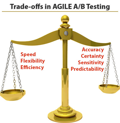
An AGILE test is no different than other approaches in the fact that the design process is in its essence all about trade-offs, compromises between the different parameters. If one wants greater certainty, one should be prepared to pay for it by an increase in the number of committed users and the longer time to get results. If one prefers to have more flexibility, then the trade-off is uncertainty of the final sample size, which in some cases may result in larger sample sizes compared to an inflexible fixed-horizon test. Thus is the nature of reality, thus is the nature of statistics.
See this in action
Advanced significance & confidence interval calculator.
For the more statistically-inclined, the design stage of an AGILE A/B test is in essence a Group Sequential Error Spending Design with Stopping Rules for both Efficacy and Futility (GSTEF) adapted to the practice of Conversion Rate Optimization for websites, applications, e-mails, etc. The analysis stage includes procedures that compensate for the bias introduced by the interim analyses to the naive versions of three popular estimators: p-value, confidence intervals and point estimator for the lift. This allows decisions and actions to be maximally informed.
In using AGILE we have several choices for trade-offs to make, with the first five being exactly the same as in a fixed-sample design test.
1. Choosing a satisfactory statistical significance level, based on how comfortable one is with committing a type I error – rejecting the null hypothesis when it is in fact true. In CRO AB testing this is how strong of an evidence you require before the new variant is implemented in the place of the existing one. (complete guide to statistical significance in A/B testing)
How high the evidence threshold needs to be can be informed by things like: is the decision reversible; how easy it would be to detect the error at a later point; how hard or how costly it would be to revert the decision once it is implemented and other considerations of that nature. There is a trade-off here due to the positive relationship between the level of certainty and the sample size – the more certain one wants to be, the more time and users one needs to commit to the experiment.
Usually a small and agile team (e.g. a startup) working on a site with a relatively small number of users can be satisfied with a lower confidence threshold (higher error rate) since the risk of doing something wrong will not have that great of an impact while the decision to reverse can usually be made quickly and easily. On the contrary – a business with a complex site or app with lots of users and revenue and a large team behind it is justified in being much more careful and requiring higher evidential support before a change is introduced, especially if it is a core change versus a superficial one.
Other considerations also come into play, such as continuity and reliability of the customer experience. The “two steps forward one step back” approach might look good in terms of long-term performance on paper, but might actually be much worse than going step-by-step in the right direction, if the disturbances and unevenness of the user experience have a detrimental longer-term effect on the business.
2. Choosing a minimum detectable effect size is to be done with commercial viability in mind. The minimum detectable effect should justify running the test and should be non-trivial in this sense. It should be the difference one would not like to miss, if it existed.
In the case of websites where redesigns and changes happen frequently we propose to consider the monthly or yearly effect, multiplied by 24-48 months or 2-4 years.
E.g. if the minimum detectable effect is set at 2% relative improvement, then multiply the yearly number of conversions by 2% and then by 2 in order to calculate the final effect of the experiment if it is successful. This can guide the decision on whether to commit a given resource in terms of users to running the test or not. There is, of course, an inverse relationship between the effect size and the sample size required to detect it with a given certainty, so a trade-off is inherent in the approach.
As Jennison and Turnbull (2006) [8] state on the problem of how to choose the effect size at which to specify the power of a clinical trial when there is disagreement or uncertainty about the likely treatment effect: “Our conclusion when there is a choice between a minimal clinically significant effect size and larger effect sizes that investigators hope to see is that the power requirement should be set at the minimal clinically significant effect. This decision may need to be moderated if the resulting sample size is prohibitive, bearing in mind that a good sequential design will reduce the observed sample size if the effect size is much larger than the minimal effect size.” By “observed sample size” they mean the actual sample size that one would end up committing, should it turn out that the true effect size is significantly larger than initially estimated. In general, if the sample size is prohibitive, reconsider the utility of running the test at all.
Smaller sites with less revenue should generally aim at more drastic improvements, otherwise the cost of running the test might not be justified. On the other hand, very large sites can aim to detect very small improvements as these are likely to correspond to a significant lift in absolute revenue. Of course, this depends on the nature and effort required to perform the test, as well as other factors, not subject to the current article.
3. Choosing a satisfactory power level is as important as choosing the significance level and the effect size, but sometimes underestimated in practice. The more powerful the test, the more likely one is to detect an improvement of a given size with a specified level of certainty (if such exists in reality). Thus the greater the sensitivity of the test, the bigger the sample size required.
The decision on the power of the test should be informed by the potential losses of missing a true effect of the specified size, the difficulty and costs involved in preparing the test and how costly it is to commit x% more users into the test. When test preparation is long and difficult or when increasing the sample size is cheap then power should be kept relatively high. (complete guide to statistical power in A/B testing)
4. Choosing how many variants to test against the control. The more variants one tests, the more things can be tested at once, though it comes at the cost of increasing the required total sample size.
5. Choosing the type of sample size / power calculation when there is more than one variant tested against the control. The two types are disjunctive (OR) and conjunctive (AND) power. In 9 out of 10 cases an AB testing practitioner would chose disjunctive power, meaning that he would be satisfied with finding one positive result (rejecting at least one null hypothesis) among the tested ones. If one wants to have the same level of power for all tested variants, choose conjunctive power, although be aware that it comes at a great cost in terms of required sample size.
6. Choosing the number of interim analyses. It is best to take a look at the estimated sample size for a fixed-sample design and consider how long it would take to achieve that sample size using a prediction based on historical amount of users/sessions/pageviews for the website or app in question. The number should be adjusted so it only includes the target group of interest, e.g. by geo-location, device category, visited pages, cookie status and others. This prevents inflating the baseline by counting in users who do not really matter which can increase the sample-size requirement by multiples in some cases.
One should not be conducting tests with a duration of less than a week, due to in-week variability which may result in issues with the representativeness of the conclusions for future traffic. If, for example, the test is estimated to take 6-8 weeks, it is best to plan for at least 8 interim analyses – 1 per week. It should suffice for weekly reporting purposes and should be frequent enough to satisfy executive curiosity. So if a site has 10000 users per week who are eligible to enter a test and the maximum expected sample size is 120000 for all arms (variants), then 120000/10000 = 12 interim analyses. Setting it to 15 just to be on the safe side is generally preferred.
In some cases, one wants a higher frequency of interim analyses and that may well be warranted, however, one should keep in mind that the more interim analyses, the higher the maximum sample size gets. Maximum sample size is the maximum information that would be needed if the experiment is not stopped at any of the interim analyses. On the plus side, the more interim analyses conducted, the better the chance for an early stopping and thus the smaller the average sample size gets.
It is encouraged to check a few different design outputs to evaluate the trade-off between number of interim analyses, average and maximum sample size.
Lan and DeMets (1989) demonstrate that even when performing twice the initially planned interim analyses the type I error probability is not significantly impacted when the sample size remains fixed. The theoretical limit of the number of analyses is to do an interim after each observation, although that is not practical at all.
In our approach we adjust the boundaries based on the actual number and timings of observations and thus keep the type I and type II error probabilities under control, but this happens at the cost of increasing the sample size required for a conclusive test. This means that if the test runs to the pre-specified maximum sample size one might end up with an inconclusive result as in figure 4 below.
It might sometimes happen that many more than the initially planned interim analyses are conducted. In such cases it might be necessary to increase the total sample size, so it is encouraged to have a realistic number of interim analyses set in the design stage in order to avoid that.
7. Choosing the Time / Information fraction at each interim analysis. Usually the time and information fraction are closely correlated, i.e. at time t = 0.5 (0 < t < 1) the amount of information collected should also be about 0.5 or 50% of the maximum information.
Usually equally spaced time intervals are chosen and we do so behind the scenes as it practically does not matter due to the continuous nature of the alpha-spending functions used to calculate the efficacy and futility boundaries. No input is required from the user in our statistical calculator.
8. Choice of error-spending functions for the efficacy and futility boundaries – there are several different popular spending functions – Pocock-like, O’Brien-Fleming-like, Hwang-Shih-DeCani Gamma family, Kim-DeMets power family – all having different properties. Our AGILE A/B testing calculator currently uses the Kim-DeMets error-spending functions for both the efficacy and futility boundary construction and the interface is not complicated by the choice of other spending functions.
9. Choice of futility boundary-type – the futility boundary can be binding or non-binding with respect to the efficacy boundary.
A non-binding boundary means that alpha and beta spending are completely independent, so when the futility boundary is crossed one can still decide to continue with the experiment without inflating the Type I error-probability. This comes at the cost of increased sample size compared to the binding design, but it is generally a preferred choice, as considerations outside of data gathered might help inform the decision to stop or to continue when the futility boundary is crossed. In this design the boundary is more of a guideline, not a rule.
If the boundary is binding, then there is some chance that the experiment will stop prematurely due to futility, so we get a reduced level of type I error – alpha. Thus, we can “spend” this gain by slightly decreasing the efficacy boundary so that the alpha level is kept as specified and we gain a bit of power, which allows us to run the test with fewer users when compared to a non-binding boundary approach. However, if a binding boundary is used the experiment must stop if the futility boundary is crossed at any interim analysis point in order to preserve the desired error control properties of the test. You can read more about the effects of futility stopping on the efficiency of A/B tests in our post on Futility Stopping Rules in AGILE A/B Testing.
See this in action
The all-in-one A/B testing statistics solution
(Added Apr 27, 2018): I have subsequently developed a comprehensive overview of the costs & benefits and risks & rewards in A/B testing (not AGILE-specific) and have built a tool that will help with the balancing act, allowing you to use A/B testing to manage business risk while maximizing gains and rewards: the A/B Testing ROI Calculator.
Evaluating the Design
With the above parameters specified, our AGILE testing tool outputs a set of data which aims to help the user better understand the trade-offs involved. This data includes, for example, the expected average sample sizes at certain true effect sizes:
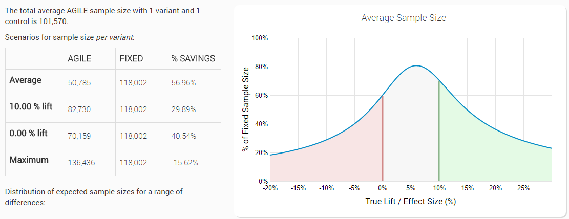
The reported design characteristics include: efficacy and futility critical values (boundaries) in a Z-scale normalized form; total sample size required in case the experiment continues through all interim analyses; expected sample size under the null and under the alternative hypothesis (if one or, respectively, the other is true, how early would the experiment terminate versus a fixed-sample design) as well as an average sample size which is calculated across a set of possible true values of the tested variant(s).
It is recommended to evaluate several designs and consider the one that suits the particular test best. There is no universally preferable set of design parameters, the same way there are no two identical tests.
We hope this post was helpful in shedding light on the practical application of the AGILE statistical approach to A/B testing. As you can see there are just a few more decisions to be made, compared to a proper fixed-horizon test, while the benefits that come from using AGILE are immense.
To learn more about efficient A/B testing, read our AGILE A/B Testing whitepaper or try our AGILE A/B Testing Calculator.
About the author

Managing owner of Web Focus and creator of Analytics-toolkit.com, Georgi has over twenty years of experience in online marketing, web analytics, statistics, and design of business experiments for hundreds of websites.
He is the author of the book "Statistical Methods in Online A/B Testing", of white papers on statistical analysis of A/B tests, and has been a speaker at conferences, seminars, and courses. Georgi has been distinguished as a winner in the Data & Analytics category of the 2024 Experimentation Thought Leadership Awards.


Is there anything wrong with designing a test like this:
1 – based on subjective opinion about the likely impact or success of the test, choose a maximum period of time over which to run the test. For example, test A is research based and I’m fairly sure it is going to be positive, so I want to give that a maximum of 8 weeks to prove itself. Test B someone else asked me to do and I don’t really believe it will work, so I an not prepared to let it hold up other tests on that page for longer than 2 weeks.
2 – based on traffic, estimate the sample size which will have been achieved at the end of that period of time
3 – design the parameters of the test in order to achieve that sample size over that period of time. If the starting point of this design is the power and confidence, then the remaining parameter to play with is the MDE, which should be as low as possible to achieve the sample size (after power and confidence set) but not lower than the cost/benefit would allow.
Therefore, what I am fundamentally doing is designing a test window of time, which is driven by my desire to move the CRO programme at pace, but I understand by doing that I will probably reject tests which might have had more subtle effects.
Hi Jonny,
The question that pops into my mind after reading your comment is: what determines what is a good pace for a CRO programme? In my mind the judgement should be based on the business bottom line, which has a rather objective correspondence to test parameters (our A/B testing ROI calculator helps enormously with that). The way I see it, the only reason to start with the time limit and work your way backwards is if there is a set deadline determined by factors external to A/B testing. Even with my experience with stats I wouldn’t trust my ability to transform any kind of judgement about the potential of an A/B test into sample size or time periods without using a tool like a power analysis calculator or, even better – the calculator cited above.
Best,
Georgi
I have run a real scenario through the ROI calculator, but after the optimisation it is suggesting the test run for 30 weeks with significance of 55% – I have yet to completely get my head around the ROI calculator, but a test which runs for potentially 30 weeks (appreciate that the point of agile is that it might not run for that time) is risky in the sense that I could have been testing something else which may have worked better. If I have 10 ideas for a single page, I can only prioritize them based on the research which gave rise to them and subjectivity, but what I want to do is find the most successful ones as quickly as possible. If I run a test for a short(ish) period of time and then discard it because it isn’t showing any evidence of positive impact, that doesn’t mean I have discarded it forever, because after I have found the stuff which is positive, I can always go back and test the other stuff for longer.
Sounds like you just need to do the math for the 10 tests you have in mind and then start with the one for which the ROI calculator suggests the shortest testing time-frame? 30 weeks is a lot, maybe you have a minuscule amounts of traffic or the changes you are making are too small to be detectable in a shorter time-frame.
Is this an appropriate use of a non-inferiority hypothesis? a HiPPO has asked me to make a fairly trivial change to the website. I could make the change quickly, and it probably won’t have much effect on anything, but I want to check it doesn’t have any negative impact. So I am not so much interested in whether it is better, just that it isn’t worse?
Maybe you meant this comment for another post, but yes, that sounds like a good situation for a non-inferiority test.